Computer Generated Images as Mathematical Tools

Liesbeth De Mol

Laboratory of Applied Epistemology, University of Ghent

e-mail: elizabeth.demol@ugent.be

Abstract

Since the commercialisation of the computer, it became possible to visualise certain aspects of mathematics that were not possible to visualise before because of the complexity or the size of the datasets involved. Some of these computer generated images even have become the icons of certain mathematical theories like for example fractal geometry. One of the advantages of these visualisations is the fact that in using them, certain properties that involve complexity can be immediately shown. This possibility will be discussed through experiments done by the author.

1. Introduction

Everybody else took an exam in algebra and complicated integrals, and I managed to take an exam in translation into geometry, and in thinking in terms of geometric shapes.

(Mandelbrot in an interview)

The computer created new possibilities for scientific research. One of these possibilities is the visualisation of certain aspects of mathematics. These computer generated images however are not only interesting as visualisations, but can also be used as instruments for doing research. More specifically, they can help researchers to answer certain structural questions i.e. questions concerning the large scale behaviour of a given system and the structure that follows from this behaviour [See for example 1, 2 and 3]. That these images can be used as research techniques is in part due to their directness i.e. you can gain knowledge of a systems’ structure just by looking at it. Especially when large or complex systems are involved, visualising the structure of the behaviour of a system can be a much more direct and quick first answer to certain specific questions. Of course this does not always imply that there is also a rigorous explanation for the properties observed, but you at least know where to start i.e. you know what the behaviour is. During recent research done by the author, this method of using computer generated images as testing tools for certain structural questions, was used [See 4]. It will be shown how this method can work in practice, together with its advantages and disadvantages.

2. Deriving fractals from IFS-systems

One of the prototypical examples of the use of computer generated images in mathematical research is fractal geometry. There are many different methods to generate fractals, depending on what kind of fractal one wants to be visualised [See 5]. In the experiments 2-dimensional IFS attractors were generated through a variant of the chaos game. An IFS-fractal is defined through a set of transformations k, which determine how a given point (x, y) is transformed into another point (x₁,y₁), where:

x₁ = aix + biy + ei (i = 1, 2,...,k; {a,b,c,d} є [-1, 1])

y₁ = cix + diy + fi

These transformations then define an attractor i.e. every point in space will be attracted by the limit figure. Using such transformations, one can generate fractal figures. One of the methods to do this is the chaos game. The chaos game is played as follows. Consider for example the following IFS-transformations:

f₁ (x, y) = (0.5x, 0.5y)

f₂ (x, y) = (0.5x + 0.5, 0.5y)

f₃ (x, y) = (0.5x, 0.5y + 0.5)

We then have to choose an initial game point (x₁, y₁), say (10, 10) and then generate a random number z₁ between 1 and 3, being the number of transformations. Depending on whether z₁ is 1, 2 or 3, we perform the first, second or third mapping respectively on the initial point, and then plot the newly calculated point (x₂, y₂). In the same way, the following transformation is determined by a newly generated random number z₂, and is then performed on (x₂, y₂), so that a new point (x₃, y₃) is calculated and plotted... When iterating this procedure for several times a visual representation of a famous fractal is generated, namely the Sierpinski triangle, which can be seen in Fig. 1.

Fig. 1 Image of the Sierpinski triangle.

Now it must be remarked that when looking at the behaviour of an arbitrary point in applying the chaos game on it, this point will have a unique orbit when following it in its convergence to the attractor. On the other hand, it must also be noticed that besides this, every point has its own convergence speed: some points will need two iterations of the chaos game before reaching the attractor, others three,...Now given these observations, the following question can be posed: given the diversity of convergence speeds and individual orbits, is there a general structuring principle behind this diversity? To answer this question, one has to be able to compare the individual orbits and speeds of these points in space, and thus find a way to observe the large scale behaviour of one group of points in space, according to their orbits and speeds. To observe how space is possibly structured according to these individual orbits, the following experiment was set up. First of all a 3816 × 2319 array of points was selected as being the points of which the behaviour was to be analysed. The attractor is located somewhere at the centre of this array. Secondly, to each point the same random string was assigned. This string consists of all the numbers between 1 and the number of transformations which define the attractor. For the Sierpinski triangle for example, this string consists of the numbers 1, 2 and 3. This string is then to be interpreted as the successive sequence of transformations to be performed when playing the chaos game. Each point (x, y) is then transformed according to this same sequence of mappings, until it reaches the attractor. At every step in this transformation the Euclidean distance d between the point and the transformed point is measured. The total distance D(x , y) = d1 + d2 + ...+ dn, where n equals the number of iteration steps needed for a specific point to reach the attractor. In applying this procedure, to every point in the array a number is assigned, which is to be interpreted as the convergence distance from a point to the attractor, following the transformations determined by the random string. Using this number, a colour can be assigned to each point. When there is indeed a structuring principle behind the individual orbits of points, we should expect that when performing this procedure, the colours will not be distributed at random, but should display discrete transitions, forming structures. In Figs. 2-4 examples are shown of applying this method to three different attractors.

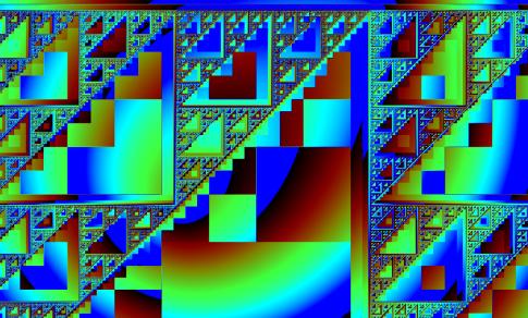
Fig. 2 Application of the method discussed. The attractor used is the Sierpinski triangle, which is framed in black here. As can be observed, this original attractor is part of a greater Sierpinski-like structure.

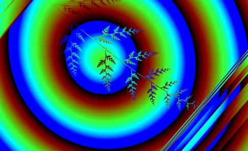
Fig. 2 Here the method is applied to Barnsley’s fern. Again one can observe that the original attractor – again framed in black – is one leaf of a greater fern.

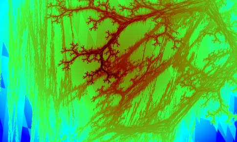
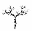
Fig. 4: Application of the method discussed, the attractor having a tree-like structure. This original attractor is the small, dark little tree which is here again framed.

As can be concluded from these computer generated images it is clear that despite the individualness of the orbits, there is clearly an ordering principle behind these orbits. One can clearly observe that groups of neighbouring points form clusters, cfr. the discrete transitions in the colouring due to discrete transitions in convergence distances. Moreover, some of these clusters resemble the original IFS-fractal, which is framed in black in Figs.2-4. When looking at the overall structure it even seems to be the case that this original attractor is part of one greater fractal structure. So one can conclude that, even if each point has a unique orbit under the transformations, there is clearly a structuring principle which classifies these points in fractal clusters. In trying to find an explanation for this clustering, further experiments have shown that this structuring is caused by the number of iteration steps to be performed on each point before reaching the attractor. When plotting only the points with a given speed, the images immediately show that each structure is indeed formed by points which have the same number of iteration steps. This is illustrated in Fig. 5 where one such structure was isolated from Fig. 4, by plotting only those points with speed 2.

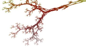
Fig. 5: Visualisation of only those points that converge to the attractor after the application of the first two mappings determined by the random string, used in Fig. 4.

Several other experiments were performed to further analyse the convergence behaviour of points when applying the chaos game on them, like for example measuring the fractal dimension of these structures, but these will not be mentioned here [see 4]. What is of more importance here is the fact that these experiments clearly illustrate how computer generated images indeed can be useful instruments for doing research. In the experiments done here, they gave an immediate answer to a question concerning a possible structural property of a system. Once such a question is solved in this way, it is often the case that the results can be further applied for different purposes. This was also the case for the results described here.

3. Applications

The fact that points in space, which are each transformed according to the chaos game using the same random string, are fractally clustered together according to convergence speed, can now be further applied for other purposes. Two kinds of applications will be discussed here.

3.1. Graphical Applications

As could be already noticed in Figs. 2- 4 the procedure described generates a fractal structure of which the attractor that is used to generate this fractal is just a small part. In this way the method can thus be used to expand an attractor. However if one wants to use this as a technique it is not enough to just perform the operation that was described, since it is clear from the figures that this expansion seems to go on without bound. This can be avoided in using the observation that these structures are formed according to convergence speed. When isolating structures according to speed, it was observed that the structure formed by points with speed 1 will form an expansion of the original attractor, points with speed 2 will form an expansion of the points with speed 1 and thus an expansion of the original attractor,... Thus to expand the original attractor one just has to add the further restriction to the algorithm that only those points with speeds smaller than a chosen value should be plotted.

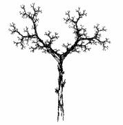
Figs. 6 The left figure shows the original attractor, while the picture on the left shows a plot of the original attractor, together with the points of speed 1. This whole structure is a scaled up reflection of the original attractor.

In Fig.6 this was done for the tree-like fractal used in Fig. 4, using a different random string. The left figure shows the original attractor, while in the figure on the right the attractor is plotted together with the points with speed 1. This plot results in a scaled up reflection of the attractor.

As a further graphical application, which was found through observations made during the experiments, the possibility of generating contours of the original attractor should be mentioned. It could be observed in Fig. 5 that when isolating a structure according to speed, the result indeed resembles the original attractor, but one part of the plot is less dense then the other part. This less dense part, is formed by points which are in the direct neighbourhood of points with speed 1. When looking at the structure formed by points with speed 1, the same is observed: the plot is divided into a dense and a less dense part. Here the less dense part is in the direct neighbourhood of the attractor. Using these observations it is possible to generate the fractal contour of an attractor. In Fig. 7 the result is shown for the tree-like fractal:

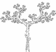Fig. 7: Plot of points with speed 1 and 2, that are in the direct neighbourhood of the attractor.

Concluding, one can say that in using computer generated images as research instruments it is possible that as a side-effect of the observations made, other techniques for generating computer images become apparent.

3.2. Theoretical Applications

We have seen that when analysing the chaos game according to convergence speeds, Euclidean space is fractally differentiated. One of the further observations made was the fact that using different random strings, results in very different visualisations. This procedure is thus sensitive to initial conditions. In slightly modifying the method these observations can be used to find typical visual representations of strings belonging to a certain class of strings. The classes of strings that were investigated are strings that are produced by systems of tags. Tags were first defined by Emil Post [See 6] and are defined in the following way. Consider an alphabet A = {α1, α2,..., αn}, over which an initial string I of arbitrary but finite length is defined, and a constant natural number v. For each letter of the alphabet we then define a corresponding non-empty string. Depending on the first letter of the initial word, the respective sequence of letters is then tagged at the end of the string, and the first v letters are removed. In this way a new string is produced, and the operation of tagging and removing letters can be repeated. Post discusses the following very simple example:

A = {1, 0}; 1 → 1011; 0 → 00; v = 3

Then choosing for example the following initial condition “1011000100010101110” the following sequence of strings is produced:

1011000100010101110

10001000101011101011

010001010111010111011

00101011101011101100

.............................................

Despite their seeming simplicity, tag systems are in general undecidable. Practically this means that given a tag that seems undecidable, its behaviour is unpredictable. One of the undecidability questions that are related to tags is the following question: given an arbitrary string, will it ever be produced by a given tag system. The research done by the author on this subject is not yet completed, but in trying to approach this problem in a more experimental way, the method here discussed was used in the following way. Given for example the above discussed tag system developed by Emil Post, and an arbitrary initial condition. When visualising the strings according to the above discussed method, one cannot find any generality in the images determined by these strings. Each string results in a different picture. This problem can be overcome as follows. Given the binary permutations of a given length n, for example the 32 permutations of length 5, one can analyse a string according to the yes or no presence of each of these bit strings in the string. Then a list is made of these bit strings that are part of the string. Using then for example the IFS-transformations that result in the tree-like fractal, the transformations to be performed are now determined in the following way. The first transformation to be performed is determined by the first bit-string in the list. This bit string is converted to its decimal value, and then divided by the number of IFS-transformations, in this case 5. It is then the remainder of this division that determines the transformation to be performed, since this remainder varies between 0 and 4. For example, when the bit string 101100 is the sixth bit string of such a list, the sixth transformation to be performed is then the remainder of the division of the decimal value 44 of this bit string by 5, which is 4. In this way a string produced by a tag is thus transformed into a new string consisting of digits varying between 1 and the number of IFS-transformations. This modification however is not enough so as to get a complete visual representation of a string produced by a specific tag. This is due to the fact that when looking at the maximum convergence speeds these are rather low. The maximum speeds in Figs. 2-4 are respectively 15, 9 and 13. This implies that when using this procedure for the transformed strings, only the first 15, 9 and 13 digits respectively will be represented in the visualisation of the string. To overcome this problem, two attractors instead of one can be used. Without going into the details of how this is done, experiments have shown that we can now have a complete representation of a tag string, reaching maximum speeds which equal the number of bit strings a tag string is analysed in. In fig. 8 the result is shown of applying this procedure for an arbitrary chosen string produced by the tag discussed by Post, for a random initial condition. The question then is if this visualisation can indeed be called a typical visualisation of this tag. This is indeed what seems to be the case.

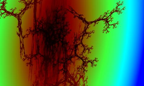
Fig. 8: Typical visualisation of a string produced by Posts’ tag, through the method discussed.

The procedure was tested for this tag for ten different random initial conditions. For each of these initial conditions, 300000 strings were produced, out of which 10000 randomly chosen strings were analysed. The results of this analysis for permutations of length 5, resulted in 0,0237% deviating strings i.e.strings that dot not result in the visualisation shown in Fig. 8. This means that there is a very small chance that strings produced by this tag will not result in the visualisation of Fig. 8, so it can indeed be called a typical visualisation of this specific tag. Moreover, when applying this same procedure to other tags, which were selected through an algorithm which tests for possible undecidability, the ‘typical’ visualisations for each of these tags was always different for each tag, so that this method can be generalised to other tag systems. Without going further into the details of the research already performed in this context, one can conclude then that this method is at least a practical answer to one of the undecidability problems that are related to tags, be it a probabilistic one. Perhaps further research on this subject can find other methods for tag recognition. In spite of the unavoidable undecidability, it can then be possible to increase the probabilities in complementing these methods with the method here discussed.

4. Conclusion

Using computer generated images as research instruments is indeed one of the interesting possibilities that became available to scientific research with the commercialisation of the computer. It is clear that these images as images are not enough on their own to perform research. The right questions have to be asked and one must be able to perform the right experiments and to interpret these results. Notwithstanding these remarks, speaking from my own experiences as a non-mathematician, it must be noticed that, as a technique, it offers the possibility of performing research in a more intuitive way. Sometimes one can get frustrated for not knowing the right mathematical formulations for found results, but most of the time, I was able to answer my questions by performing new visual experiments.

References

[1] Martin Gardner, The fantastic combinations of John Conway's new solitaire game "life” in: Scientific American, 223, 1970, 120-123.

[2] Stephen Wolfram, Random Sequence Generation by Cellular Automata in: Advances in Applied Mathematics, 1986, 123-169.

[3] Benoît Mandelbrot, Les Objets Fractals: Forme, hasard et dimension, Paris:Flammarion, 1995.

[4] Liesbeth De Mol, Study of Fractals derived from IFS-fractals by Metric Procedures, submitted to Fractals.

[5] H.Peitgen, H.Jurgens and D. Saupe, Chaos and Fractals. New Frontiers of Science. Berlin: Springer Verlag, 1992.

[6] Post, E. L. Formal Reductions of the General Combinatorial Decision Problem. In Amer. J. Math. 65, 197-215, 1943.