New methods for the three-dimensional representation

of high-dimensional objects

Philip Van Loocke

Abstract. The paper develops new methods for the visualization of high-dimensional objects. An algorithm minimizing different kinds of error functions is described. The contrast between metric and structural adequacy is illustrated. Aesthetic representations of hypercubes are obtained in the metric domain if different types of structure are integrated, and in the structural domain when spatially bifurcating curve sets are taken as a point of departure. Then, a weighted sum of vertex-based transforms is associated with the visualization of a hypercube. These transforms construct map from Rⁿ onto R³ on basis of the visualization of a hypercube. This is illustrated for four-dimensional objects generated by a function familiar from fractal contexts.

1. Introduction

The question how high-dimensional structures can be visualized in three dimensions has been raised since the advent of non-Euclidean geometry and of modern physics (Kaku, 1994; Barrow, 2003), and has inspired several artists (Henderson, 1983). Toward the end of the nineteenth century, knowledge about the conceivability of a fourth dimension spread, among others, in England and in France. From about 1910, cubist art was often explained as a means for the artist of expressing a four-dimensional reality. Artists such as Duchamp explicitly tried to develop new methods for visualizing the fourth dimension. They embedded their practice in a more global philosophical view on a four-dimensional universe. It was influenced by Russian authors and artists (such as Ouspensky and Malevitch), who linked four-dimensional concepts with a mystical attitude, which was linked with platonism. In the United States, ideas about higher dimensions widely spread through literature, such as the science fiction of Wells. Through the work of Bragdon, four-dimensional concepts found their way to the design of ornaments. In the twenties, Buckminster Fuller brought these ideas into the field of architecture. But although there are notable exceptions, the four-dimensionalist artistic/philosophical inspiration and interest faded after 1920.

In the past few decades, this interest gradually re-emerged, because computer technology gave new opportunities for visualizing high-dimensional objects. Popular work on computer graphics, like the book of Banchoff (Banchoff, 1990), brought these possibilities under wider attention. Digital architecture included the concept of higher dimensions in its design process, such as in the work of Novak or Lalvani (Lalvani, 2003).

In this paper, new methods for obtaining computer generated visualizations of high-dimensional objects are constructed. In section 2, a stepwise algorithm for visualizations of n-dimensional hypercubes is explored. The algorithm is run for metric constraints, and for structural constraints that are cast in metric terms (section 2). Subsequently, the algorithm is reformulated in terms of branching structures. This yields representations in which different types of three-dimensional spatial structures are combined. Section 3 comments on the difficulty of reconciling structure and metric in the representation of high-dimensional objects. As an alternative to a stepwise procedure, section 4 describes a structural approach that generates forms of a more organic nature. Finally, section 5 describes how the visualizations of hypercubes can serve as a basis for a transform of the entire space Rⁿ onto R³. The transform is illustrated with visualizations of some four-dimensional structures defined in quaternion space.

2. A stepwise algorithm for two and three dimensional visualizations of hypercubes

Consider a hypercube in n dimensions. It has 2ⁿ edge points or ‘vertices’, which are denoted P_i. Suppose that the hypercube is mapped on a two- or three-dimensional visualization. The point on which P_i is mapped is denoted Q_i. The vertices P_i are supposed to have coordinates equal to –1 or +1. The coordinates of Q_i take continuous values and are adapted in the course of the stepwise algorithm.

Suppose that the coordinates of Q_i are initialized randomly. The Euclidean distance d(Q_i,Q_j) for all couples of points (Q_i,Q_j) is determined, and this quantity is normalized by division by the largest value found for it: d*(Q_i,Q_j)=d(Q_i,Q_j)/d_max, where d_max is the maximal distance between points Q_i and Q_j. Similarly, in the hypercube, all n-dimensional Euclidean distances d(P_i,P_j) between edge points are determined, and normalized by division by 2.n^(1/2): d*(P_i,P_j)=d(P_i,P_j)/ 2.n^(1/2) (for the given choice of coordinates, 2.n^(1/2) is the largest distance between different edge points in the hypercube). Then, the error measure E₁ = S_{{i,j=1,…,n}} (d*(Q_i,Q_j)-d*(P_i,P_j))² can be used to measure the metric resemblance between the hypercube and its visualization. It is proportional to a measure known as ‘stress’ or ‘Sammon error’ in the literature on data visualization.

A stepwise algorithm minimizing this error can be defined as follows. The points Q_i are give random initialization. At each step, one point Q_j and one dimension in the visualization are selected randomly. The quality e.a is added to the coordinate of Q_j along this dimension; e is the stepsize of the algorithm, and a is a random number between –1 and +1. If the new coordinates of Q_j lead to a lower value of E₁, the change in coordinates is kept; else, the old coordinate values are restored. Different runs of this algorithm generally yield different visualizations, though the final value of E₁ is often the same. Figure 1 shows a two-dimensional visualization of a three-dimensional cube (with E₁=1.904); Figure 2 illustrates a two-dimensional visualization of a four-dimensional cube (with E₁=11.946).

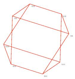
Figure 1. Two-dimensional visualization of a cube by minimization of E₁

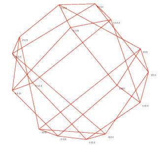
Figure 2. Two-dimensional visualization of a hypercube with n=4 and for minimization of E₁

The visualization of the hypercube in Figure 2 lacks symmetry. Symmetry is restored when the algorithm is applied for three dimensional visualizations. This is illustrated in Figure 3, where two representations corresponding to n=4 are shown (in both cases, E₁=3.769). The visualizations obtained show point-symmetry relative to the center of the Q_i-structure. The left and the right part of Figure 4 show a representation of a five, respectively a six-dimensional hypercube (with E₁=24.102 and E₁=120.378). The point-symmetry of the visualization remains for n=5 and n=6.

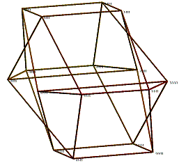
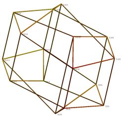
Figure 3. Two visualizations of hypercubes for n=4 and for minimization of E₁

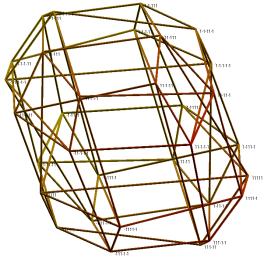
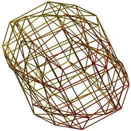
Figure 4. Visualizations of hypercubes for n=5 (left) and n=6 (right)

Consider the smallest squares on the surface of the hypercube. These squares are determined by edge points {P_i1,…,P_i4} for which n–2 coordinates take the same value, and for which the remaining two coordinates form the four combinations (–1, –1), (–1,+1), (+1, –1) and (–1,+1). The number of such squares is equal to s(n) = 2^n-2. B(n, n–2), where B denotes the binomial value. Similarly, the smallest 3-dimensional cubes are formed by sets of different edge points {P_i1,…,P_i8} which have the same value along one dimension. The number of such cubes in the hypercube is c(n) = 2^n-3. B(n, n – 3).

The four edge points of a smallest square define (4² – 4)/2 = 6 different distances. For the j-th smallest square, the k-th distance between edge points is denoted ds_jk. Similarly, for every smallest cube, the eight edge points define (8² – 8)/2 = 28 distances; dc_jk is the k-th distance relation associated with the j-th cube. The largest distance that occurs in a smallest square is 2^(1/2); in case of a cube, the corresponding value is 3^(1/2). Similar distances can be determined also for the images Q_i of the edge points P_i in the visualization. Suppose that d’s_jk is the k-th distance between the points in {Q_j1,…,Q_j4} on which the square {P_j1,…,P_j4} is mapped. Similarly, d’c_jk is the k-th distance between points on which the edge points of the j-th smallest cube are mapped. The largest distance in d’s_jk (k=1,…,6), respectively d’c_jk (k=1,…,28), is denoted d’s_j,max, respectively d’c_j,max. With these notations, two additional error functions can be defined:

E₂= S_{{j=1 to s(n)}} S_{{k=1 to 6}} (ds_jk/2^(1/2) – d’s_jk / d’s_j,max )²

E₃= S_{{j=1 to c(n)}} S_{{k=1 to 28}} (dc_jk/3^(1/2) – d’c_jk / d’c_j,max )²

Error function E₂ measures how well smallest squares in a hypercube are mapped on squares in the visualization. E₃ measures how well the visualization preserves distance relations for smallest cubes. Figure 5 shows two examples of two-dimensional solutions found for minimization of E₂ and for n=3 (and with E₂=12.618 and E₂=8.657). For n=3, E₃ coincides with E₂. Figure 6 shows a visualization of a hypercube with n=4 and for minimization of E₂ (E₂=22.952). In Figure 7, E₃ is minimized (E₃=21.661). Three-dimensional visualizations are shown in Figures 8-11. Figure 8 has two examples of visualizations for n=4 and minimization of E₂ (E₂=12.394 and E₂=12.200). Figure 9 shows two examples for minimization of E₃ (E₃=12.629 and E₃= 12.618). The left, respectively the right, form in Figure 10 gives a visualization for n=5 and minimization of E₂, respectively E₃ (E₂=53.965 and E₃=80.735). Finally, in Figure 11, the left, respectively the right part, illustrates the case n=6 for minimization of E₂, respectively E₃ (E₂=173.245 and E₃=365.124).

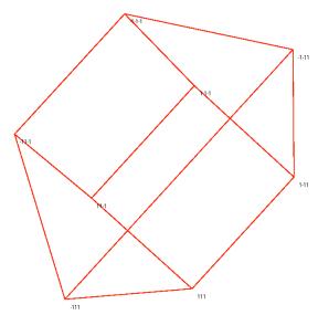
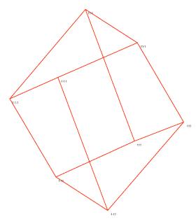
Figure 5. Two visualizations for cubes obtained by minimization of E₂

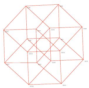
Figure 6. Two-dimensional visualization of a hypercube for minimization of E₂

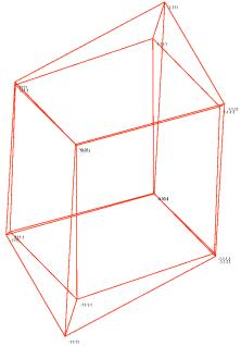
Figure 7. Two-dimensional visualization of a hypercube for minimization of E₃

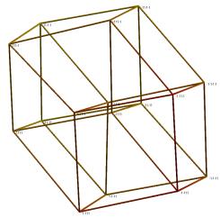
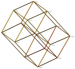
Figure 8. Three-dimensional visualization of the hypercube for n=4 and minimization of E₂ .

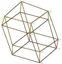
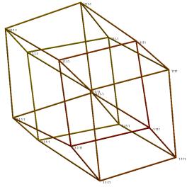
Figure 9. Visualization of the hypercube for n=4 and minimization of E₃

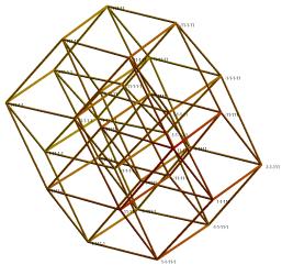
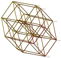
Figure 10. Visualization for n=5 and minimization of E₂ (left) and E₃ (right)

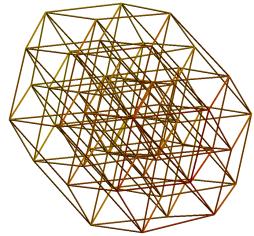
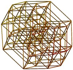
Figure 11. Visualization for n=6 and minimization of E₂ (left) and E₃ (right)

3. Angular variables corresponding to a branching process

In the previous section, the search algorithm varied Cartesian coordinates of edge points Q_i. For a different choice of variables, the points Q_i can be obtained by a spatial branching process consisting of n subsequent bifurcations. At the first stage of the bifurcation process, two branches with starting point in the origin are defined. The endpoint of a branch is the starting point for two new branches at the next level, until, at stage n, 2ⁿ endpoints are generated. Each branch is characterized by two angles f and q, and by a length l, where f is the angle between the horizontal projection of the branch and the x-axis, and q is the angle between the branch and the z-axis. The angles f and q can be adapted by the stepwise algorithm of the previous section, for any of the functions E₁, E₂ or E₃. This yields a system with 2. (2+…+ 2ⁿ) angular parameters. In the examples in Figures 12-13, branches were given length inversely decreasing with the branching level.

The configuration to which the branching system converges lacks symmetry, but the endpoints of the branches have point-symmetry. This accords with the fact that the value of E₁ in these examples approximates the values found in section 2 (in Figure 12, E₁=3.801, and in Figure 13, E₁=24.503). The algorithm can be run for symmetrically constrained branching systems. In this case, half of the tree is constructed as a point-mirror of the other half, and the total number of parameters is divided by 2. Then, solutions with higher E₁-values are obtained. This is illustrated in Figures 14-15, where symmetry was imposed, resulting in E₁-values 10.757, 12.624 (Figure 14) and 65.002, 48.916 (Figure 15). The illustrations are for branches of constant length (except for the first two branches, which were given shorter length).

These visualizations of hypercubes have a special aesthetic property. The tree-structure in itself has no clear interpretation to an observer not informed about its purpose. In Figures 14-15, the visualization of the hypercube, when drawn apart from the underlying tree-structure, is also of limited appeal (since the E₁-value is relatively high, the fact that a hypercube is being visualized is not apparent). But by matching the tree-structure with the with the visualization of the hypercube, each type of three-dimensional structure can be interpreted with help of the other.

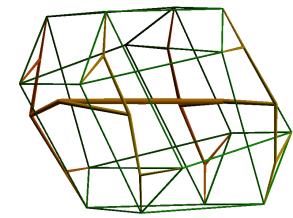
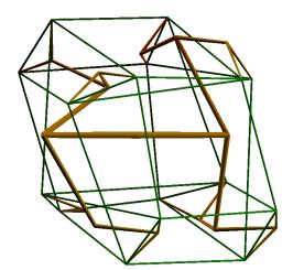
Figure 12. Two examples for angular variables and with branches of decreasing length

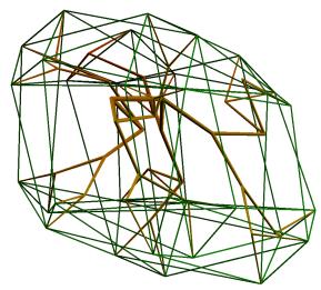
Figure 13. Visualization of the five-dimensional hypercube for angular variables

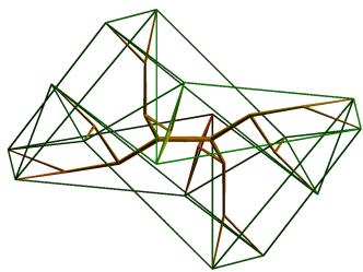
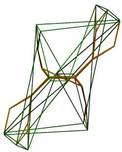
Figure 14. Visualizations of hypercubes with point symmetry imposed

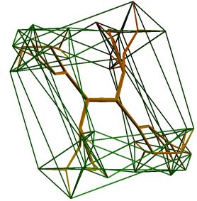
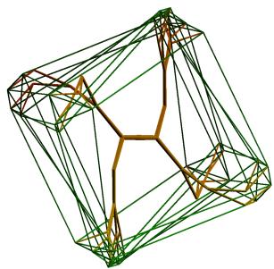
Figure 15. Visualizations of hypercubes (n=5) with point symmetry imposed

The branching algorithm can be run in a sequential way. First, a visualization for n=2 (corresponding to the visualization of a square) is computed. The 2³ additional branches required for the visualization of the cube (corresponding to n=3) are attached at the endpoints of the branches corresponding to n=2. During the search corresponding to n=3, the latter are kept fixed. This process is continued. At the k-th step, the angles associated with the 2^k new branches are allowed to vary. This results in a fast algorithm when compared to a non-sequential procedure. Such an algorithm was run several times. Branching structures with systematicity were never found, in the sense that angles between branches at later stages were not related in any systematic way to angles between branches at previous stages. This was not helped if different dimensions were given different weight in the metric function. Suppose that the coordinates of P_i, respectively Q_i, are denoted x_i^k (k=1,…,n), respectively y_i^k (k=1,2 or k=1,2,3). In Figure 16, the error function E’₁ = S_{{i,j=1 to N}} (dⁿ(P_i,P_j)/d_max – d³(Q_i,Q_j)/d’_max)², with dⁿ(P_i,P_j) = (S_{{k=1 to n}} ((1/k).(x_i^k–x_j^k)) ²) ^(1/2) and d³(Q_i,Q_j) = (S_{{k=1 to 3}} ((1/k).(y_i^k–y_j^k))²)^(1/2) was used. As a consequence, each additional dimension led to a smaller deformation of the metric relations obtained at a previous stage.

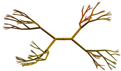
Figure 16. Tree-visualization for n=7 and with E’₁ = 126.390

The lack of systematicity limits the aesthetics of the branching forms. Structural properties appear to be hard to reconcile with metric constraints, and this difficulty increases as n increases. For values of n higher than 6, representations which are visually accessible, or which have aesthetic symmetry, can still be obtained if the metric procedure is replaced by structural considerations.

4. Structural visualizations of high-dimensional discrete spaces

The spatial branching process used in section 3 can be generalized into an alternative visualization procedure based on structural considerations. As a point of departure, a rectangular parallelepiped is constructed with sides b.g, b.g² and b.g³ (g<1). This structure is turned into a visualization of four-dimensional hypercube by splitting the smallest side-surfaces into two smaller rectangles with sides b.g⁴ and b.g⁵ (see Figure 17). Then, the new rectangles split again in two smaller rectangles to yield a representation of a five-dimensional hypercube, and so on. For splitting processes with appropriate structural properties, aesthetic representations result.

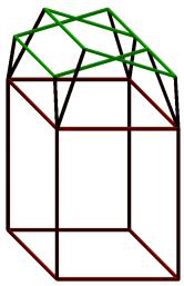
Figure 17. Splitting the upper side-surface of a rectangular parallelepiped

An instance of a splitting process is defined as follows. We confine the definition to the splitting process at the top rectangle of the cube (so that half of the visualization of the hypercube is generated; the other half is obtained by mirroring the resulting structure relative to the horizontal plane).

The first three binary dimensions of the n-hypercube are associated with the edges of the parallelepiped. Then, two curves are constructed, corresponding with fourth component values +1 and –1, respectively. The curves are defined as successions of t line segments. The starting point of the curves is the middle of the upper rectangle of the parallelepiped. The angles j and q of the segments linearly increment according to the rule: dj=c.x₄ and dq=d.x₄, where x₄ is the fourth component value associated with a curve. The new rectangles are attached on top of these curves. They are obtained by scaling the top-surface of the parallelepiped, and are orthogonal to the segment on top of which they are drawn. The length of a line segment in a curve is multiplied with a factor z (z <1) at each step, so that the bifurcating curve structure has smaller branches after each new bifurcation.

After the rectangles corresponding to the fourth dimension are drawn, each of the curves splits into two new curves. The change in angles of the segments in the curves remains determined by dq = c.x_k and dq = d.x_k (k³5). This process is continued until k equals n. In order to allow endpoints to be located in different horizontal planes, at each odd step in the bifurcation process, the value of q is increased by an amount k at the initial segment corresponding to x_k = 1 if x₄ = 1, and at the initial segment corresponding to x_k = -1 if x₄ = -1. In order to prevent the branching structure from curling too strongly onto itself, the parameter k is defined as a decreasing function of k. More specific, in the illustrations in Figures 18-19, k=k_c(n+1-k)². Figure 18 shows the upper part of the visualization of a 13-dimensional hypercube for c=0.0175, d=0.0175, z=0.993, and k_c=0.125. Figure 19 shows the underlying curve structure for variation of one parameter in the construction (d=0.0105). Figure 19 was drawn with continuous circular contours in order to ease visual track of the bifurcation process.

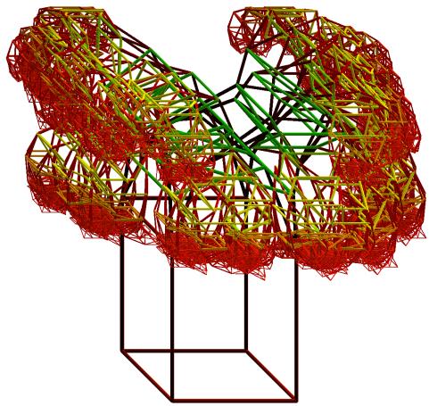
Figure 18. Upper part of a structural visualization of the thirteen dimensional hypercube

Figure 19. Example of an underlying bifurcating curve set

The aesthetics of bifurcating curve sets can be studied in its own right. For different parameters, and for a constant value of k, a binary tree corresponding to ten bifurcations is shown in Figure 20. The end-points of this structure are associated with a binary, ten-dimensional space. The procedure can be defined for p-ary spaces. The nature of the curve sets generated can be made more general also by giving the rules for dj and dq a more general form. This is illustrated for a ternary space, and for which x_k can take values –1, 0 and +1 in Figures 21-25 (k=1,…n; since we only illustrate the branching curve structure, k can start at value 1 instead of at value 4). Suppose that dj and dq are defined in accordance with dj = c.f(j,q).x_k and dq = d.g(j,q).x_k (c and d are constants; also k is kept constant in the illustrations which follow). If f and g are well chosen, end-points of branches develop in non-co-planar ways and with aesthetic spatial symmetry. The parameters and functions in these rules can be tuned toward a visually accessible representation of a p-ary space, or toward representations of aesthetic interest.

The definition of f and g is facilitated if the angles j and q are drawn into the interval [0,p/2]. Two angles µ and n are considered; µ is obtained from j by subtracting iteratively p/2 from Abs(j) until a number in [0,p/2] is obtained; n is obtained in the same way on basis of q. Then, the form in Figure 21 is obtained for f=-µ and g=n (Figures 21-24 show branching structures with endpoints corresponding to the points of a seven-dimensional ternary space). The form in Figure 22 results with f=µ² and g=1-n. Figure 23 is obtained for f=8µ^(1/2) and g=-n^(1/2) . Figure 24 corresponds f=µ⁴ and g=µ⁴. Figure 25 is made for a ternary eight-dimensional space and for f(m)=-m^1/2, and g(n)=8n^1/2.

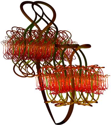
Figure 20. Form associated with a space of ten binary dimensions

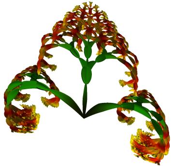
Figure 21. Form with f=-µ and g=n

Figure 22. Form with f=µ² and g=1-n

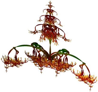
Figure 23. Form with f=8µ^(1/2) and g=-n^(1/2)

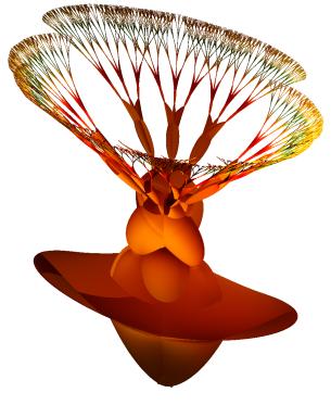
Figure 24. Form with f=µ⁴ and g=µ⁴

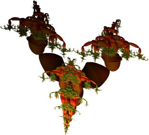
Figure 25. Form corresponding to an eight-dimensional ternary space

In Figures 20-25, the curve-structure was enveloped with non-circular volumetric elements. For each curve, circles were drawn around the end-points of all line segments, and orthogonal to the curve. In case of a ternary space, for each line segment, there are two corresponding segments on alternative curve-continuations and which belong to the same stage in the bifurcation process. An enveloping circle was elongated in the direction of these alternative continuations. The resulting contours were connected by lines.

5. Transforms constructed as weighted vertex-based functions

The previous section aimed to obtain visualizations for high-dimensional spaces by exploration of the structural instead of the metric domain. This section returns to the metric visualizations of section 2. Instead of visualizing hypercubes, a general transform F: Rⁿ ® R³ is described which visualizes arbitrary high-dimensional objects. The transform takes a

visualization of the hypercube as its point of departure, and maps a point in Rⁿ on a point in R³ as a function of its metric and angular relations with the vertices (or ‘edge points’) and the edges (or ‘side-lines’) of the hypercube. The visualizations obtained by the algorithm of section 2 generally do not correspond to linear projections of the hypercube. Therefore, the function F which embeds objects in the visualization is also not linear, although usually only ‘weakly’ so.

The transform F is defined as a weighted sum of angular vertex-based transforms. With each vertex of a hypercube, an angular vertex-based transform f_k(x) is associated as follows (k=1,…,2ⁿ). The unit vector originating in the center of the hypercube and pointing to the k-th edge point is denoted e_k (k=1,…,N). The components of e_k are equal to 1/n^(1/2) or –1/n^(1/2). The unit vector pointing from Q_k to Q_r in the visualization is denoted v_kr. With these notations, f_k: Rⁿ ® R³ associated with vertex P_k is defined as follows:

f_k(x) = Q_k + s. |x–P_k| . (S_{{r=1,...,N; r¹k}} (e_r. (x–P_k)/ |x–P_k| ) . v_kr) / c

with:

c= | S_{{r=1,...,N; r¹k}} (e_r. (x–P_k)/ |x–P_k| ) . v_kr |

The function f_k(x) contains a distance factor |x-P_k| and a directional factor (S_{r=1,...,N} (e_r. (x–P_k)/ |x–P_k| ) . v_kr) / c. Due to the normalization, the directional factor specifies a unit vector in R³. The distance factor entails that the distance between f_k (x) and Q_k in R³ is s times the distance between x and P_k in Rⁿ, from which it follows that f_k(P_k)=Q_k.

Figure 26 illustrates an edge-based transform for n=4 and for the point Q₁ in the Q_k-structure in the first form in Figure 8. The Figure shows the transform of a 12x12 grid defined over the four-dimensional hypercube. All points on the grid were transformed according to f₁(x) (with s=1.05. a/b, where a is the average distance between edges in the P_k-hypercube, and b is the average distance between different points Q_k). It can be observed that, in the neighborhood of Q₁, the transformed grid approximates a linear grid structure coinciding with planes through Q₁ and the neighbors with which it forms a smallest square. The quality of the approximation decreases for points which are images of points removed from P₁ in the hypercube.

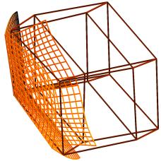
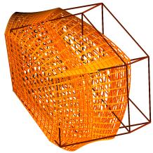
Figure 26. Vertex-based transform operating on the side-planes of a four-dimensional hypercube containing Q₁. The left figure shows the transforms of the side-squares containing Q₁. The right figure shows the transform of the entire side-square structure.

A good approximation of an overall linear structure over the Q_i-structure is obtained if vertex based transforms for all points P_i are summed into a weighted combination. The function F is obtained if a transform f_k is given a weight proportional to a power r of the inverse distance between x and P_k:

F(x) = (1/c). S_{{k=1 to N}} f_k(x) / |x-P_k|^r

with

c= S_{{k=1 to N}} 1 / |x-P_k|^r

Figure 27 shows the result of F(x) when applied to the same Q_k-structure as in Figure 26. It can be noticed that the voted sum turns local approximations into global approximations (the Figure was generated for r=1; this property remains for other visualizations of the hypercube, and for values of n higher than 4; a study of this fact was carried out in Van Loocke, 2003).

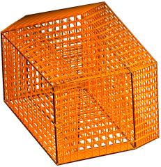
Figure 27. F(x) operating on the side-squares of the hypercube

The function F(x) can be used to obtain visualizations of any n-dimensional form. In Figures 28-33, it was applied on a generalization of a function familiar in a fractal context.

Suppose that a four-dimensional point x has coordinates x₁,…,x₄. Then, the quaternion expression f(x)=x²+c has four components f₁,…,f₄ which are defined by f₁(x)=x₁²-x₂²-x₃²-x₄²+c₁, f₂(x)=2x₁²x₂²+c₂, f₃(x)=2x₁²x₃²+c₃, f₄(x)=2x₁²x₄²+c₄. The following procedure defines a function g(x). First, f(x) is iterated t₁ times. The result of this function, but with the first component transformed in its negative, is used as input for t₂ additional iterations of f, after which the first component is changed into its negative again. The resulting point is uniformly contracted toward the origin, except for the first coordinate, which is displaced by an amount a. This cycle of t₁+t₂ iterations is repeated t₃ times. The resulting point is g(t₁,t₂,t₃;x). In Figures 28-33, gg(t₁,t₂,t₃;x) was applied to a square 27x27-grid defined over a structure defined over the four-dimensional hypercube which was contracted uniformly to the origin by a factor h. In Figure 28, h =0.333, t₁=2, t₂=1 and t₃=3. In Figure 29, the same parameters are used, but F is applied on basis of a different visualization of the hypercube. In the next Figures, these parameters were h =0.333, t₁=3, t₂=2 and t₃=3 (Figure 30); h =0.333, t₁=3, t₂=4 and t₃=3.(Figure 31); h =0.333, t₁=5,t₂=4 and t₃=4 (Figure 32); h =0.0121, t₁=5, t₂=5 and t₃=6 (Figure 33); h =0.0121, t₁=5, t₂=5 and t₃=8 (Figure 34).

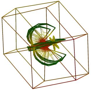
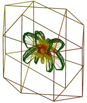
Figure 28 (left) and Figure 29 (right)

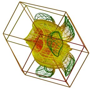
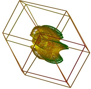
Figure 30 (left) and Figure 31 (right)

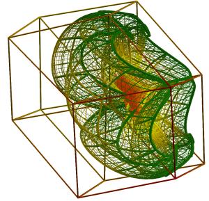
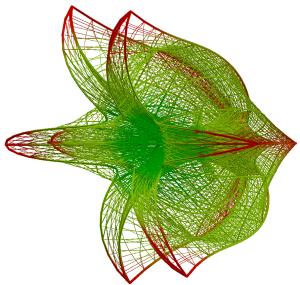
Figure 32 (left) and Figure 33 (right)

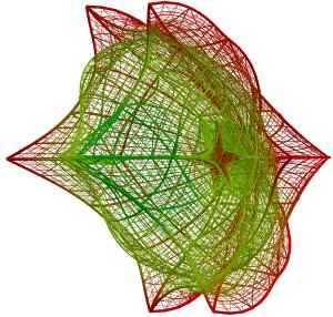
Figure 34 (left) and Figure 35 (right)

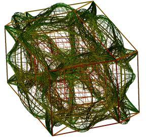
Figure 34 (left) and Figure 35 (right)

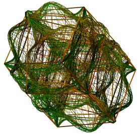
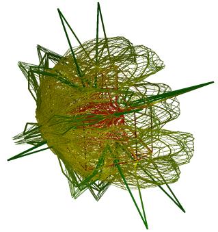
Figure 36 (left) and Figure 37 (right)

Variations of F(x) can be obtained in several ways. In Figures 35-36, F(x) was applied on the side grid over the hypercube, but for functions f_k(x) in which the factor s|x-P_k| was replaced with s|x-P_k|.(1+sin(5|x-P_k|)). In Figure 37, this strongly non-linear transform was used to map the side grid after it had been transformed by the procedure used in 28-34, and for h=0.4, t₁=1, t₂=1 and t₃=4.

6. Conclusion

The paper considered visualizations of high-dimensional objects. As a point of departure, visualizations were used which came out of stepwise algorithms. The tension between metric accuracy and desirable structural properties was discussed. In section 5, a non-linear projection method was developed to obtain visualizations of high-dimensional objects matched in the visualization of a hypercube. In other work, the latter method was applied to data-visualization and was compared with principal component analysis, which corresponds to the selection of a well-chosen linear projection. It was pointed out that, for different real-world data-sets, the metric accuracy of a visualization based on the non-linear transformation F was better than the metric accuracy of principal component analysis (Van Loocke, 2003). This is part of the motivation for using F instead of linear projections in section 5.

References

Banchoff, T. (1990), Beyond the third dimension, New York: Scientific American Library

Barrow, J. (2003), The constants of nature, from alpha to omega, Pantheon Books

Henderson, L. (1983), The fourth dimension and non-Euclidean geometry in modern art, Princeton University Press

Kaku, M. (1994), Hyperspace. A scientific odyssey through parallel universes, time warps and the tenth dimension, Oxford University Press

Lalvani, H. (2003), Genomic Architecture. In (Eds. Gans, D. and Kuz, Z.) The Organic Approach to Architecture, Chichester: Wiley Academy, pp.115-126.

Van Loocke, Ph. (2003), Application of weighted vertex-based transforms to data visualization (submitted)