Symbolic organic design

Philip Van Loocke

Art and Consciousness Studies, University of Ghent, Belgium

e-mail: philip.vanloocke@ugent.be

Abstract

We propose a method for organic construction in which hypercube visualizations are grown by trees. The growth process corresponds to stochastic gradient descent on a multi-dimensional scaling error surface. The local minima of the surface correspond to trees which are bent in such a way that their endpoints define hypercube visualizations. The surface has much more local minima corresponding to solutions of different visual appearance than dimensional scaling based on variation of coordinates, which is an advantage from the artist point of view. Additional constraints are included in the error function in order to increase the design relevance of the local minima. The method proposed includes symbols, such a hypercubes, in organic design. From this perspective, it is complementary to approaches which include visual elements from the environment in generative design.

1. Introduction

The hypercube is a symbol for one of the fundamental properties of our universe; for this reason it has attracted many artists in the course of the past century [1]. In the past few decades, computer graphics further enhanced the interest in visualizations of high dimensional structures. After the pioneering work of Banchoff [2], artists like Robbin gave visualizations of hypercubes a prominent place in their work [3]. These days, visualizations of four-dimensional polyhedra are used at many congresses to illustrate the link between mathematics and art. With the advent of 3D-printers, high dimensional structures have been used to generate three-dimensional art (see for instance the work of Bathsheba Grossman [4]). This paper aims to hint at the possible use of such concepts in a context of organic architecture.

In the work which is described below, the hypercube symbol takes a central place. It is grown by trees which are ‘symbolic’ too in the sense that they are not copied from real trees in nature. This symbol-oriented approach to design is complementary, for instance, to Soddu’s work in organic architecture [5]. In the latter, organic constructions are realized by genetically recombining elements taken from the real, visual environment. Here, we modify the code of plants so that they express symbols, which are in people’s minds, instead of in their physical environment.

2. Multi-dimensional scaling in a tree based parameter space

Multi-dimensional scaling is one of the core ingredients of our method. It is an algorithm that searches for representations of high-dimensional objects which are metrically as accurate as possible. Consider a four-dimensional hypercube. Suppose that its sixteen vertices P_r have coordinates p_r,i, with r=1,…,16; i=1,…,4. The Euclidean distance between the r-th and the s-th vertex is d_r,s= (S_i=1,…,4 (p_r,i–p_s,i)²) ^(1/2). Suppose that d_max is the largest distance between vertices. In order to apply MDS, all four-dimensional distances are normalized by division by d_max.

Consider a three-dimensional visualization of this hypercube. Suppose that the vertices in the visualization are denoted Q_r, and that their coordinates are q_r,j, with r=1,…,16; j=1,…,3. The Euclidean distance between the three-dimensional representations of the r-th and the s-th vertex is d’_r,s = (S_j=1,…,3 (q_r,j–q_s,j)²) ^(1/2). Also here, all distances are normalized by division by the largest distance d’_max. Then, the MDS error function E₁=S_{r=1,…16,s=1,…16} (d_r,s–d’_r,s)² quantifies the difference between the metrical relations in the three-dimensional visualization and the metrical relations in the four-dimensional object.

MDS starts with a random initialization of the points Q_r. The value of E₁ which is associated with this initialization is calculated. Then, a stochastic algorithm is used in order to incrementally minimize E₁. At each time step, small variations of randomly selected coordinates q_r,j are considered. If the variations led to a lower value of E₁, the new coordinates are kept; else, the old values are restored. For this procedure, the lowest value of E₁ that we obtained was E₁ = 3.769. Figure 1 illustrates a visualization which corresponds to this value. We notice that the solutions found by MDS are not linear projections of the four-dimensional hypercube on a three-dimensional subspace. This is illustrated by the fact that the edges (or ‘side squares’) in the visualization are not perfectly plane structures (see for instance the upper left part of Figure 6c below; since edges are not flat surfaces, their intersections can be curved instead of straight lines).

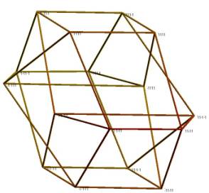
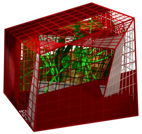
Figure 1. Hypercube visualization corresponding to a local minimum of E₁

We also worked with a second error function E₂, which expresses how well the eight side-cubes of the hypercube can be recognized in the three-dimensional visualization. Each side-cube is defined by eight vertices. For each side cube, the distances d_k,r,s between pairs of vertices are calculated (k=1,..,8, r=1,…,8, s=1, ..8; the index k refers to the side-cube; r and s refer to vertices which participate in the k-th side-cube). The distances are normalized by division by the largest distance which occurs in a side-cube. The same quantities are calculated for the three-dimensional visualization, yielding distances d’_k,r,s. Then, E₂ is given by E₂= S_{k=1,…8, r=1,…8, s=1,…8} (d_k,r,s–d’_k,r,s)². In visualizations which are based on this error function, cube-like features are more easily detectable, at the expense of lower overall metrical resemblance to the four-dimensional hypercube.

The second ingredient of the present method is a particular type of three-dimensional tree. We apply MDS not on coordinates of loose points, but on points which are attached to trees. During the MDS search process, the location of the points is varied by bending the trees, and by stretching its branches in a systematic way. A tree has a starting point Q⁰. At this starting point, the first bifurcation occurs: two branches split off, with endpoints Q¹₁ and Q¹₂. At both endpoints, two new branches appear. The endpoints of the new branches are Q²₁, Q²₂, Q²₃ and Q²₄. The branching process is iterated two more times until, at the fourth level, 16 branches result with endpoints Q⁴₁ ,…,Q⁴₁₆ (see Figure 2).

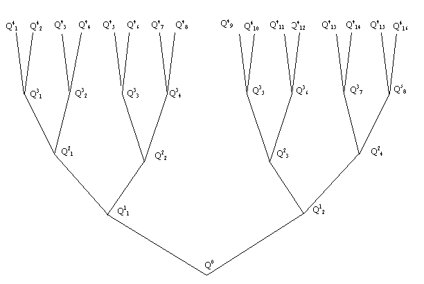
Figure 2. The structure of the tree. It is bent in three dimensions until the endnodes coincide with the vertices of a hypercube visualization.

The tree in Figure 2 is only a schematic representation of the tree which we use. We use trees which we use are curved in three dimensions. In Figure 3, we give an example of a three dimensional tree which we used as an initialization for the search process. In earlier work, we studied trees of this type which were bent by fractal fields. In order to give an idea of the type of visual representation that can be obtained in this way, we include a further illustration in Figure 3. It shows the five highest levels of a ternary tree with eight branching levels. The tree was initialized in such a way that its endpoints coincided with points on the Sierpinski triangle. Then, a fractal process was used to define the curvature of its branches (for a general description of this method, we refer to [6-7]).

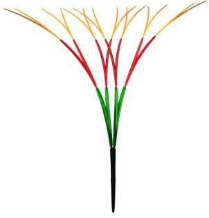
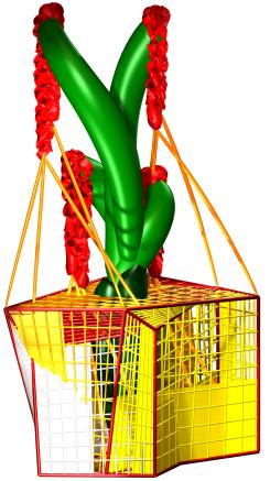
Figure 3. Initialization of the tree.

In this paper, we will not bother the reader with a technically detailed description of the parameters which are associated with a tree. In total, 42 continuous parameters are associated with the curvatures of the line segments of which branches are composed. These parameters are chosen in such a way that the symmetry in Figure 3 is only partially broken. For instance, the projections on the horizontal plane of all branches of the same level with odd index have the same curvature. A similar point holds for branches with even index. Also, the angles between the z-axis and corresponding line segments of different branches of the same level take the same value. The fact that symmetry is broken only partially is important if we want to obtain representations of aesthetic quality. Four additional parameters are associated with the length of the branches. At each level, all branches with odd index are allowed to expand by the same amount. All branches with even index are contracted by this amount. The total number of parameters that is associated with a tree, and that is varied in the course of the search process, is therefore equal to 46. This is comparable to the number of parameters in an ordinary MDS algorithm. In the latter, each three-dimensional point which represents a vertex is varied. Since such a point has three coordinates, 16 x 3 = 48 parameters are subject to variation.

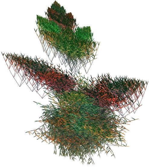
Figure 4. Example of a ternary tree with eight branching levels (only the last five ones were included in the Figure)

Whether run on basis of error function E₁ or E₂, the tree search algorithm is able to find solutions with the same error value as ordinary MDS. It also often finds solutions corresponding to local minima of higher error. Since these are sometimes remarkable from an aesthetic point of view, for the computer artist it is of relevance to explore also the latter. Due to the inclusion of the trees, the number of local minima which correspond to different visualizations is much larger for the present algorithm than for ordinary MDS.

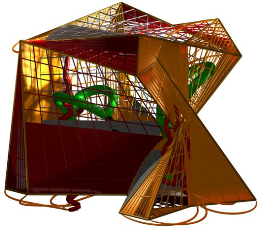
In Figures 5a-b, we present two solutions found by the search algorithm. The first Figure was obtained for E₁, the second for E₂. They illustrate that the algorithm sometimes converges to a relatively strongly bent tree. This can be encouraged if the variations during the initial steps of the search process are allowed to take large values. Though these representations are often remarkable, in most illustrations which follow below, we have chosen trees which hide the hypercube visualization to a lesser extent.

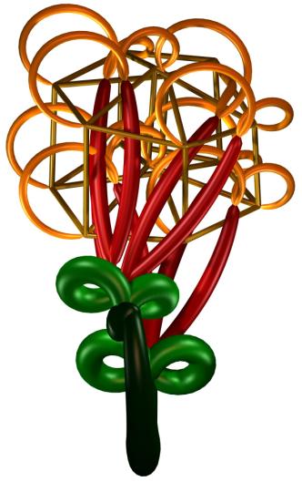
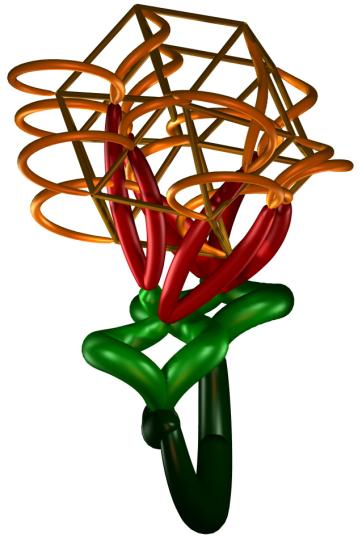
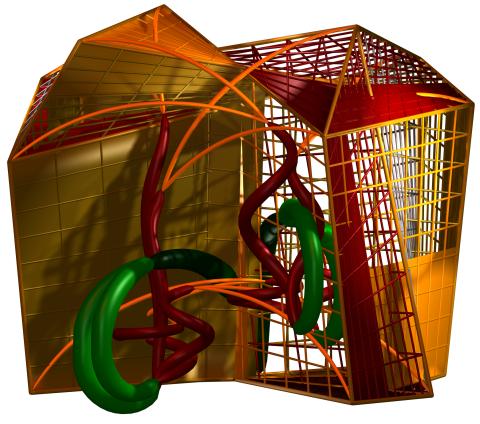
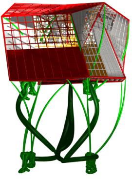
Figure 5 a-b. Solutions obtained for E₁ (Figure 5a) and E₂ (Figure 5b)

The structure of a hypercube visualization can be made clearer if we fill all or some of its 24 edges. We implemented three methods to visualize edges. The first method covers edges with a grid of some thickness. The second one covers the entire edge with a surface. Third, half of the surface of an edge can be filled, which has the advantage of still allowing partial visual access to the structure behind the edge. We rendered our visualizations in Microstation. The options for visualizing edges were put in different ‘levels’ of this software. This means that they were included or excluded in the visualization with a single mouse click. Figures 6a-e include five illustrations. The upper three were obtained by stochastic gradient descent of the error surface defined by E₁, the lower two correspond to local minima of E₂.

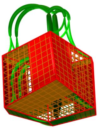
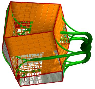
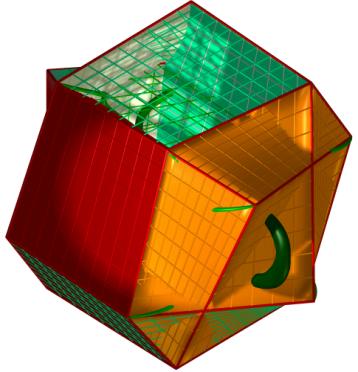
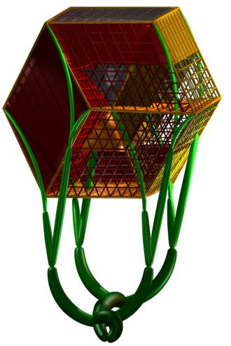
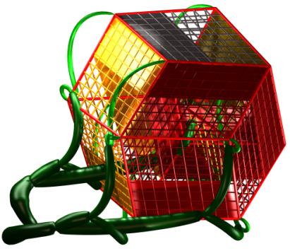
Figure 6a-e. Five examples of solutions. The upper three were obtained by minimization of E₁, the lower two by minimization of E₂.

3. Constraints which increase the design relevance of solutions

While contemplating forms like in Figure 6c, we wondered if we could modify the error landscape in such a way that the solutions would hint at organic architectural designs. For instance, if the visualizations of the hypercubes have a relatively broad horizontal basis, they have more stability from a constructive point of view. Also, from this perspective, the tree has a more natural place if its starting point belongs to the plane defined by this basis.

In order to include these constraints in the search process, we selected six vertices in the hypercube visualization. For each of the vertices, we calculated the distance to the horizontal plane in which the starting point of the tree was located. The sum of these distances was added as a penalty term to the error function. As a result, the local minima of the new error function have a horizontal base in which the visualizations of at least these six vertices are located, and which has the same altitude as Q⁰. Trees were allowed to partially grow below this plane. In some solutions, also part of the hypercube visualization led to a ‘basement’ below this plane (see Figure 7a).

The search algorithm can be modified also by changing the variables by which trees are characterized, or by increasing the degrees of freedom for the curvature of the branches. In the illustrations of the previous section, angular differences between successive line segments of the same branch were required to take constant value. For the illustrations for this section, we included eight more parameters which allow branches to curl in more sophisticated ways. The inclusion of more parameters entails that the error surface is defined over a space with more dimensions. As a result, also the number of local minima is further increased, which practically means that the variety in shapes produced by the search process increases too. We include eight illustrations in Figures 7a-h. All Figures correspond to local minima of the modified E₂ error surface, except for Figures 7c and 7f, which are two views of one solution on basis of the modified E₁ error function.

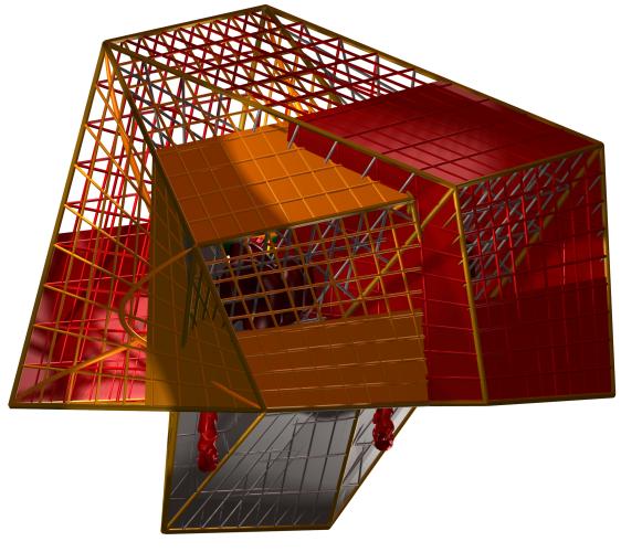
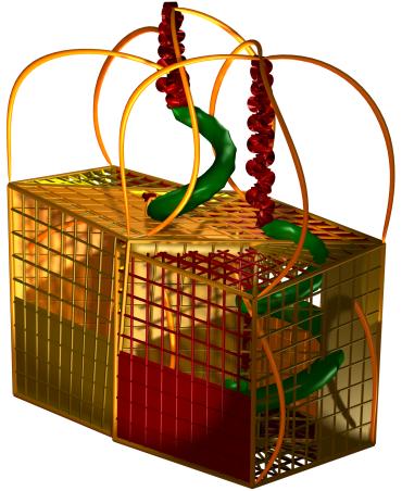
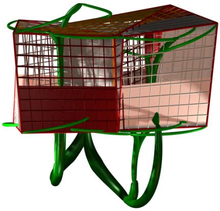
Figures 9 a-h. Eight illustrations of solutions obtained for the modified landscape

4. Comparison with a direct method

The organic forms of the previous section can be contrasted with the structures which result from a more direct approach. For this end, we wrote another piece of code which gives the user the choice of locating the edges of the hypercube. Once an artist has acquired familiarity with hypercube visualizations, it becomes straightforward to locate the edges in such a way that a large base, as well as a horizontal first floor, and a relatively simple roof structure, fit into the whole (see Figure 10). Afterwards, a tree can be constructed so that its endpoints coincide with the vertices of the hypercube visualization.

The direct approach leads to forms which are easily constructible. But there is a price to pay. The organic quality of the whole is inferior to the one of the visualizations of the previous section. In special, it is hard to conceal that the tree structure did not really define the location of the vertices. We notice that the preference of humans for organic forms has been extensively documented (see [8]). This preference is not limited to the aesthetic domain. In the field of environmental psychology, much evidence has been collected which demonstrates that organic environments reduce stress, with several positive side effects [9] (this is also one of the reasons why studying organic and fractal forms in educational settings has been advocated [10]). The technical challenge of realizing constructions based on the forms of the previous section is higher than in case of constructions obtained by the direct method, but it may be more rewarding, both from an artistic and a broader humanistic point of view.

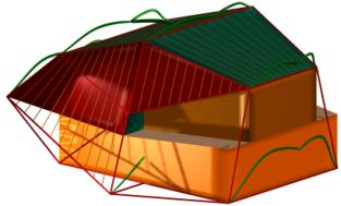
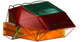
Figure 10 a-c. Two views of the same house obtained by the direct method

5. Discussion

In this paper, we described how organic design can be guided by the desire to include symbols, such as the hypercube symbol. Symbols of this type are culturally universal. All people who are scientifically contemplating the physical structure of our universe, or cosmology, see the same universe, and use the same mathematical symbols. But as was demonstrated in Soddu’s work, one of the strengths of generative design is that it allows one to integrate visual elements which reflect the soul of cities, which is very culture specific. The present method is complementary, but not contradictory to this approach. In future work, we hope to develop a hybrid method, in which visualizations of universal symbols are cast into a design methodology that is flexible enough to refer to visual patterns of cultural specificity.

References

[1] Henderson K (1983) The fourth dimension and non-Euclidean geometry in modern art. Princeton University Press, Princeton

[2] Banchoff T (1996) Beyond the third dimension. Geometry, computer graphics, and higher dimensions. Freeman and Company, New York

[3] Robbin T (1992) Fourfield. Computers, art and the fourth dimension. Bulfinch Press, New York; see also tonyrobbin.home.att.net/

[4] see www.bathsheba.com/

[5] see www.generativedesign.com/

[6] Van Loocke Ph (2004) Visualization of data on basis of fractal growth. Fractals 12(1): 123-136

[7] Van Loocke Ph, Joye Y (2006) Symmetry breaking in fields as a methodology for three-dimensional fractal form generation. Computer and Graphics 30(5) (about to appear)

[8] Joye Y (2005) Evolutionary and cognitive motivations for fractal art and art and design education. The international Journal of Art and Design Education 24(2), 175-185

[9] Ulrich R (1993) Biophilia, biophobia and natural landscapes. In: Kellert S, Wilson E (eds) The biophilia hypothesis. Island Press Washington, pp 73-137

[10] Joye Y, Van Loocke Ph (2006) Systems theory and organic construction. Motivation and educational perspectives. Systems Research and Behavioral Science 23 (about to appear)