Generative flowers and flower canopies as visualizations of binary information and of DNA sequences

Philip Van Loocke

Lab for Applied Epistemology, University of Ghent

philip.vanloocke@Ugent.be

Abstract

A set of three-dimensional branching structures is defined. The endpoints of trees are associated with p-bit strings. Coefficients associated with p-bit strings determine the local curvature of the branches. Long bit-strings are analyzed in terms of shorter p-bit strings, and the coefficients thus obtained map long bit-strings on a visualization in terms of a tree-structure. The tree-visualization is turned into a flower-visualization by definition of a non-linear tree-based projection. As an alternative, the flower-visualization is attached multiple times at the endpoints of the tree. The distribution of coefficients of p-bit strings determine the spread of the flower canopy, the size of flowers, and the open/closed-attribute. Interpolation of bit-strings yields interpolation of the corresponding flower-visualizations.

Keywords: visualization, bit-string, non-linear projection, generative flower, Mandelbrot set

1. Introduction

The beauty of plants and trees has inspired much work in computer graphics [1]. Fractal approaches to generative tree construction have been applied to data-visualization by different authors [2-6]. Typically, such approaches analyze data in a hierarchical way, so that they can be mapped on a bifurcating tree. The components of the data which are most important according to a formal analysis (such as an entropy method, or principal component analysis) are mapped on the initial nodes of the tree; less important components guide data through subsequent bifurcations until the leaf-level is reached. This paper visualizes long strings of binary and quaternary data. A string is analyzed by moving a p-bit window over it, and by determining coefficients for each of 2p or 4p strings of length p. The short strings are associated with the leafs of a tree with 2p or 4p end-nodes, and the coefficients of these strings determine the curvature in the branches of the tree.

The tree-representation that is obtained depends on an initialization. An initialization is appropriate if the spatial structure of branches gives visual information about the p-strings attached. This can be realized if the initialization of the tree is a highly structured and familiar form. The present paper uses the boundary of the Mandelbrot set to initialize trees.

After a tree is bent by data, it is turned into a flower form. This is obtained in two steps. First, endpoints are interpolated by a contour. Second, this contour is projected in a series of steps so that a surface is obtained. The projections are defined by successive small variations of the parameters associated with the tree. The length of line segments in branches is decreased, so that a form is obtained which converges toward the starting point of the tree. Depending on the choice of parameters, more concrete or more abstract flower forms result. Finally, this method is turned into a generator of flower canopies by putting the flowers on top of bent tree representations. The spread of the flowers over the leafs of the tree, as well as their attributes ‘size’ and ‘open/closed’ are based on information derived from p-window analysis.

2. Spatial trees: initialization and bending on basis of p-bit analysis of long binary strings

Two types of spatial trees are considered in the present context: binary trees in which, at each bifurcation point, a branch splits in two branches, and quaternary trees in which branches split in four new branches. The initialization of a tree is specified by the endpoints of its final branches, by the starting point S of the tree, and by a series of factors g1,…,gp, which specify to which extent branches are drawn to S at each level. In case of a binary tree, 2p endpoints Spj (j=1,…,2p) are given. In all examples which follow, these points are chosen at constant line distance on an oriented contour of the Mandelbrot-set. The endpoints are grouped in p/2 pairs of points with consecutive indexes, and for each pair, the average point S*,p-1j (j=1,…,2p-1) is determined. These points are contracted toward S by the factor gp. The resulting points are the starting points of the final level branches of the tree. This process is repeated until, at level one, two points S1j (j=1,2) are obtained. The tree is completed by connecting each point S1j with SºS0.

For a quaternary tree, the same procedure is followed. On the contour of the Mandelbrot-set, 4p points Spj (j=1,…,4p) are chosen at equal line distance. An initial point S and p factors gi are defined (j=1,…,p). At level p-1, 4p-1 points are obtained by taking averages of four consecutive points, and by contraction of the latter toward S by the factor gp. This procedure is iterated until, at level one, 4 points S1j result. These are connected with S in order to complete the tree. Figure 1 illustrates these concepts. Figure 1a shows the contour on which the endpoints are defined. In Figure 1b, a binary tree corresponding to p=8 is shown. Figure 1c illustrates a quaternary tree for p=5.

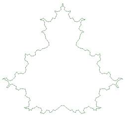
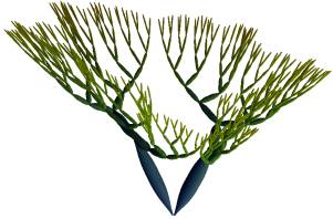
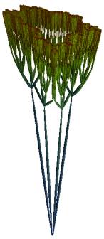
Figure 1a-c. Contour of the Mandelbrot-set with points selected for a binary tree and p=8 (Figure 1a); Figure 1b shows a binary tree for p=8; in Figure 1c, a quaternary tree for p=5 and different values for g_j is shown

In order to bend the tree, each branch is divided into M segments. Consider a sequence of p branches, starting at the first level and ending up at the p-level. Such a sequence is called a ‘long branch’; it consists of N=n.M segments. Consider the h-th segment along such a long branch, and suppose that it belongs to an s-th level branch (so that (s-1).M < h < s.n+1 and s=1,…,p). The length of the line segment is denoted l_h .The unit vector e_h along the segment is specified by two angles (q_h, j_h), where q_h is the angle between the x-axis and the projection of e_h on the horizontal plane, and j_h is the angle between the z-axis and e_h. The difference between q_h+1 and q_h, respectively j_h+1 and j_h, is denoted dq_h, respectively dj_h: q_h+1 = q_h + dq_h and j_h+1 = j_h + dj_h. A tree will be bent by specification of modifications for the differences dq_h and dj_h.

In order to obtain trees which keep symmetry, the bending process is made a function of the order of branches in the set of two or of four branches to which they belong (where these sets are defined by the fact that branches of the same set have the same starting point). In case of a binary tree, values +1 and –1 are associated with the first, respectively the second branch of a set. In case of quaternary trees, values +2, +1, –1 and –2 are associated with the branches. Suppose that the value associated with the s-th branch in the long branch is denoted a_s. Then, a simple rule for bending the tree is obtained as follows:

dq_h= dq_h + a_s. e₁ and dj_h = dj_h + e₂

where e₁ and e₂ are constants

This rule is complemented with a second one, which inserts additional angular changes at each first segment of a branch. These changes are periodic functions of the branching level s, and also linearly increase as a function of s, in order to prevent the tree from curling into itself too strongly. In case of a binary tree, the second rule reads:

dq_h = dq_h + a_s g₁ .s. cos(a₁+b₁.s)²

If a₁= +1 and a_s = +1 then dj_h = dj_h + g₂ .s. cos(a₂+b₂.s)²

If a₁= -1 and a_s = -1 then dj_h = dj_h + g₂ .s. cos(a₂+b₂.s)²

where h = 1 + (s-1).n (s=1,…,p), and a₁, b₁, a₂ , b₂ , g₁ , and g₂ are constants

For combinations of a₁ and a_s not mentioned in the rules for j_h, no change of the difference is made. In case of a quaternary tree, the rule following rule was used:

dq_h = dq_h + ha_s g₁ .s. cos(a₁+b₁.s)²

If a₁= 2 and a_s = -2 then dj_h = dj_h + g₂ .s. cos(a₂+b₂.s)²

If a₁= 2 and a_s = -1 then dj_h = dj_h + g₂ .s. cos(a₂+b₂.s)²

If a₁= 1 and a_s = -2 then dj_h = dj_h + g₂ .s. cos(a₂+b₂.s)²

If a₁= 1 and a_s = -1 then dj_h = dj_h + g₂ .s. cos(a₂+b₂.s)²

If a₁ = -1 and a_s = 1 then dj_h = dj_h + g₂ .s. cos(a₂+b₂.s)²

If a₁ = -1 and a_s = 1 then dj_h = dj_h + g₂ .s. cos(a₂+b₂.s)²

If a₁ = -2 and a_s = 2 then dj_h = dj_h + g₂ .s. cos(a₂+b₂.s)²

If a₁ = -2 and a_s = 2 then dj_h = dj_h + g₂ .s. cos(a₂+b₂.s)²

where ha_s= 1 if a_s= +2 or a_s= +1 and ha_s= -1 if a_s= -1 or a_s= -2

The rule for quaternary trees is formulated in terms of ha_s instead of a_s in order to avoid wide horizontal divergence between branches. The second rule is not applied to the branches connecting S with the first level nodes.

The parameters in the tree-bending rules are made a function of the statistics of sets of combinations of p letters in a binary or quaternary information sequence. Suppose that a quaternary string is considered. For each combination of p letters, the number of times the combination occurs in subsequent places of the string is determined. This defines 4^p coefficients, which are associated with the 4^p p-th level branches of the tree. Suppose that such a coefficient is denoted w^p_j (j=1,…,4^p). In order to associate coefficients with lower level-branches, the coefficients w^p_j are propagated backward through the tree. For each lower level-branch at level s (s=1,…,p-1), a coefficient w^s_j is defined which is the average of the coefficients of the four branches sprouting from it (j=1,…,4^s). At each level of the tree, normalized coefficients are determined. Normalization occurs by drawing coefficients at the same level between zero and one by subtraction of the smallest value at the level, and by division by the difference between the largest and the smallest value. Normalized coefficients are denoted nw^s_j. In order to visually represent the statistics of p-combinations of letters, the quantities nw^s_j are inserted in the tree-bending process. This is realized by making the parameters e₁, e₂, g₁ and g₂ proportional to a power r of one minus the normalized coefficients nw^s_j (a₁, a₂, b₁ and b₂ are kept constant throughout the whole tree). In case of binary trees, the similar procedure is followed.

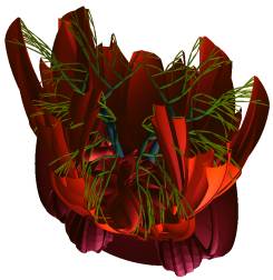
The quantities nw^s_j are generally not symmetric, so that the initial symmetry of the tree is not conserved. The aesthetics of bent tree-forms (and of the flowers enveloping them in the next section) is often significantly increased if mirror symmetry relative to a vertical plane is maintained. In order to obtain this, the coefficients of the s-th and of the 1+4^p-s -th combination of letters are replaced by their average value (s=1,…,4^p-1). This choice divides the number of statistical quantities represented in the tree by 2. This concepts are illustrated for six DNA codes which can be found on GENBANK (JCvirus, pappilomavirus, human herpesvirus 5, simian adenovirus 3, human adenovirus C, and human adenovirus B). Figure 2a-2f were generated for quaternary trees with p=8 and r=2. Figure 3a-f correspond to binary trees with p=8 and r=1. The Figures were obtained for the initialization shown in Figure 1c.

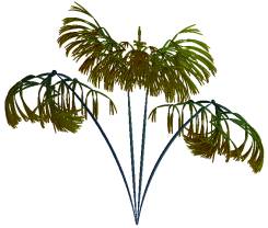
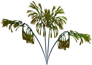
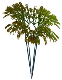
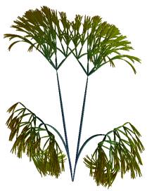
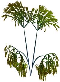
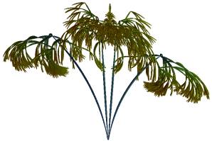
Figure 2a-f. Non-linear quaternary trees for p=5 and for JCvirus, human pappilomavirus, human herpesvirus 5, simian adenovirus 3, human adenovirus C, and human adenovirus B

3. Flowers visualizing binary and quaternary strings by non-linear tree-based projection of contours

The contour by which the endpoints of trees are initialized can be reconstructed after the bending process. Endpoints with successive indexes can be connected by a line, or can be interpolated in a non-linear, curved way. The latter option will be followed in the present paper.

Consider the line interval between end-points with indexes k and k+1. The length of the interval is notated d. Suppose that, for a given number q, G is the average point of the endpoints with index between k-q and k+1+q (if an index in this set is smaller than 1, 2^p is added to it; if it is larger than 2^p, then 2^p is subtracted from it). For each point P on the line interval, the unit vector originating in G and pointing to P is determined. Then, if d* is the distance between P and the k-th endpoint, P is displaced in the direction of the unit vector by an amount proportional to (0.5)² - ((d*/d) - 0.5)².

Once the tree is constructed, the initial contour can be complemented with a set of t-1 additional contours which connect endpoints of trees generated for different parameters. If the space between contours is filled, an object results. Suppose that, among the variations in parameters, the length of line segments decreases stepwise to zero. Then, the initial contour shrinks and is drawn to the origin, so that, when contours are interpolated, a structure results which is closed at the origin and which opens up toward the initial contour. This procedure can be used to generate concrete or abstract flower-like structures on basis of an initial contour. In the illustrations which follow, the length of line segments is contracted linearly when subsequent trees are drawn. When the sequence of contours is reversed, contours grow upward from the origin by increase of the length l of line segments according to l = l_ini.(q-1)/(t-1) (q =1,…,t), where l_ini is the length of the segment in the tree corresponding to the initial contour. This process is turned into a non-linear projection method by a) specifying that the vertical angles j of all line segments are replaced by angles c₁.j+c₂.z, with c₁=((s-1)/(t-1))^r, c₂=1-c₁, and where z is a fixed angle, and b) by linearly decreasing the impact of the data on the bending process when generating trees shrink toward the origin.

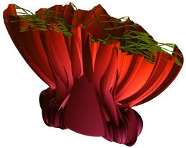
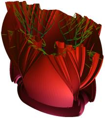
This process is illustrated for generative, binary strings in Figure 3e-f. The Figures were generated for bending parameters of weak, intermediate, an higher value. In Figure 4a-b, two DNA sequences were recoded as binary strings first, after which the corresponding flower structure was generated. In Figure 5a-b and 6a-b, two DNA sequences were visualized by quaternary trees and for different values of z.

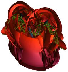
Figure 3a-b. Two flower representations of bit strings for low values of bending parameters

Figure 3c-d. Four flower visualizations of bit-strings for intermediate values of bending parameters

Figure 3e-f. Four visualizations of bit-strings for high values of bending parameters

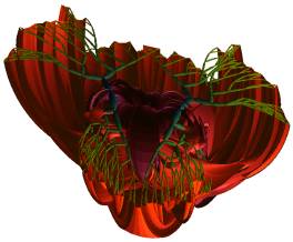
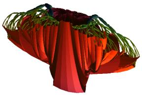
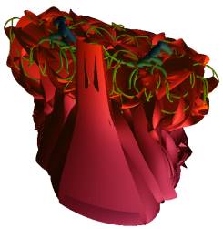
Figure 4a-b. Flower structures corresponding to binary recoded human adenovirus C and human adenovirus B

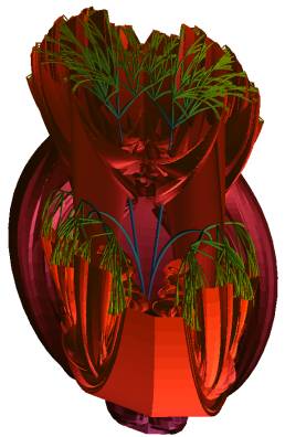
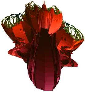
Figure 5 a-b. Flower structures corresponding to human adenovirus C and human adenovirus B

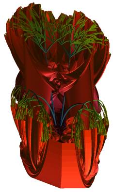
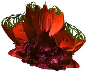
Figure 6a-f. Flower structures corresponding to human adenovirus C and human adenovirus B, and for different value of z

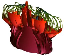
4. Flower canopies as visualizations of information strings

An object generated by the method of the previous section can be ‘fractalized’ on basis of intrinsic parameterization. On each contour in the set of non-linear projections of the initial contour, 2^p endpoints of a tree are marked. On the q₁-th contour (0 < q₁ £ t), r₁ endpoints can be selected at which a new object is attached (0 < r₁ £ 2^p). In special, the object itself can be attached in a scaled version at such a point. In the present paper, the object is rotated over an angle which is equal to the angle between the z-axis and the final line segment pointing to the endpoint. This process can be iterated. On the scaled object, the q₂-th contour can be selected (0 < q₂ £ t), and a scaled rotated version of the original object can be attached at r₂ selected endpoints (0 < r₂ £ 2^p), and so on. Figure 7 gives an illustration for an initial contour corresponding to a non-bent tree. The figure shows the initial object along with two stages of fractalization.

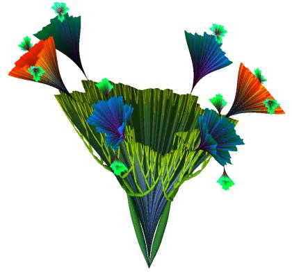
Figure 7. Form generated for non-bent tree on initial contour and with two levels of fractalization

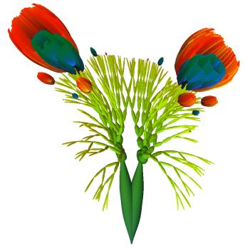
When bit-strings are visualized, the visual accessibility of a structure is enhanced if the initial object is not drawn, and if objects at the first stage of fractalization are attached at the top-contour of the initial object. As a result, a branching stem is provided with flower-structures at its endpoints. The density of the canopy can be made a function of properties of the distribution of coefficients in p-bit analysis. Suppose that q₁ sites are determined in a symmetric way so that the i-th site is symmetric relative to site 1+2.q₁-i (i=1,…,q₁). For the q₁/2 first sites, the function b(i)= 1-Abs(q₁/4-i) / (q₁/4) is calculated (Abs denotes the absolute value function; b(i) increases linearly from 0 to 1 between 0 and q₁/4; it decreases from 1 to zero between q₁/4 and q₁/2); for the q₁/2 last sites, the function b(i) is given by b(i)=1-Abs(q₁/4-(i-q₁/2)) / (q₁/4). Two parameters associated with the distribution are calculated. First, the highest coefficient c_max of p-bit strings is determined. Second, the number of coefficients which are larger than x.c_max is calculated (in the illustrations which follow, x=0.5). The square root of this number is denoted s. Then, at each of the sites i (i=1,…,q₁), a rotated version of the initial flower-structure is attached with a scale proportional to c_max.b(i)^(r1-r2.s). Since b(i) is smaller than one, a low value of s entails that a steep distribution of flowers in the canopy results and vice versa. The numbers r₁ and r₂ in the exponent of b(i) have to be chosen in such a way that, for the largest value of s in the set of strings which are visualized, r₁-r₂.s is always positive.

Along with size, the attribute ‘open/closed’ is associated with each flower. In the construction process of the flower, the quantity b(i)^(r1-r2.s) is used to modulate vertical angles of the line segments of all contour-projecting trees. More specific, the angles of all segments in the s-th tree are multiplied with a factor f given by f = (c₁+c₂ (1- (s-1)/(t-1))), where c₁= b(i)^(r1-r2.s) and c₂=1-c₁. This factor leaves angles at the bottom of a flower unaffected, and reduces angles to c₁ at the top of a flower. In order to prevent this process from being accompanied with the appearance of long peeks in the center of the flower structures, the length of all line segments can be scaled with a factor (e₁-e₂ (s-1)/(t-1)), where e₁ and e₂ are constants and e₂=1-e₁. In the illustrations which follow, e₁=0.75 and e₂=0.25. This way, the larger flowers in the Figures open up, whereas smaller ones remain closed. Figures 8-9 illustrate flowers generated for two different bit-strings, with s=3 and s=7, respectively.

Figure 8. Flower visualization of bit-string with s=3

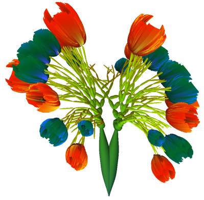
Figure 9. Flower visualization of bit-string with s=7

5. Discussion

The use of a non-circular initial contour for the trees was motivated by the fact that a contour with structure allows one to more easily visually locate a leaf corresponding with a particular p-coefficient. The association between p-coefficients and leafs was weakened by the symmetry operation to which all trees were made subject. Removal of the symmetry constraint gives trees which are more informative, but with degrading aesthetics. Since aesthetics eases visual assessment of complex representations, it was adopted nevertheless.

It can be noticed that bit-strings can be interpolated in a stepwise way. A first bit-string which differs in n bits from a second one can be turned into the latter by n successive bit clips. In the corresponding visualization, this process entails that the flower structure associated with the former gradually changes into the flower structure associated with the latter. Consider a very long bit string of length N₁, for instance a string corresponding to a long piece of music. A long window of length N₂ (with N₂<N₁) can be moved stepwise over the string with length N₁. If the string in the N₂-window is subject to p-bit analysis and visualized by the present method, then moving the N₂-window corresponds with movement in the flower visualization. In the visualization of section 4, this implies that the tree structure is transformed continuously, that the flower canopy widens and shrinks, and that flowers open and close as long as the window is moved. At this moment, this process is still too computation intensive to obtain real time visualization of music on ordinary hardware, but it offers another outlook for further continuation of this research.

References

[1] P. Prusinkiewicz, A. Lindenmayer, The algorithmic beauty of plants, New York: Springer

[2] E. Kleiberg, H. van de Wetering, J. van Wijk (2001), Botanical visualization of huge hierarchies, in Andrews, K., Roth, S., Wong P. (eds.) Proceedings of IEEE symposium on information visualization, 87-94

[3] B. Shneiderman (1992), Tree visualization with tree-maps: a 2-D space-filling approach, ACM Transactions on graphics, 11(1): 92-99

[4] H. Koike, H. Yoshihara, Fractal approaches for visualizing huge hierarchies, in Proceedings of the IEEE 1993 symposium on visual languages, 55-60

[5] J. Carriere, R. Kazman (1995), Interacting with huge hierarchies: beyond cones trees, In: Proceedings of the IEEE 1995 symposium on information visualization, 74-81

[6] P. Van Loocke (2004), Data visualization with fractal growth, Fractals, 12(1), 123-136