Density flow of a vector field along the roman surface of Steiner

Prof. E.Musso, PhD.

Dipartimento di Matematica Pura ed Applicata

Università de L’Aquila- L’Aquila-Italy.

e-mail: musso@univaq.it

Abstract

In this paper we consider the density flow of a vector field along the Steiner’s Roman surface. The components of the vector field are Wierstrass’s elliptic functions. Symbolic and numerical computations, as well the visualization, are performed with the software Mathematica 5.1.

Denisity flow of a vector field along the roman surface of Steiner

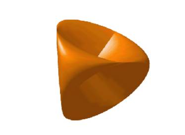
Fig. 1 : the roman surface of Steiner.

The roman surface is defined by the parametric equations

(1) x(u,v)=cos(u)²cos(v)sin(v),

(2) y(u,v)=cos(u)sin(u)cos(v),

(3) z(u,v)=cos(u)sin(u)sin(v).

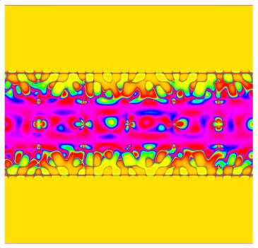
Fig. 2 : densità del flusso del campo vettoriale W

This picture represents the density of the flow of the vector field W with components

(4) W¹(u,v) = Re[σ(u+iv, ω₁+ iω₂)],

(5) W²(u,v) = Im[P(u+iv, ω₁+ iω₂)],

(6) W³(u,v) = Im[σ(u+iv, ω₁+ iω₂)],

where P and σ denote the Weierstrass elliptic functions with fundamental periods ω₁=1 and ω₂=2. The density through the surface is given by

(7) ρ = N∙W (g₁₁ g₂₂ - g₁₂²)^1/2,

where the functions g_ij , i,j=1,2, are the coefficients of the first fundamental form of the surface and N denotes the Gauss map. The visualization of the density is obtained by the means of the following “color function”

(8) CF(u,v) = Hue(-1/2(1+(1+ ρ)(1+ ρ²)^-1),1,1)

The program

The program has been written with the software Matematica 5.1.

Fig. 4: the program