Synchronized Swamp: Uncanny Expressive Mathematics

Pierre Proske, MSc, BE, BA

IT University Göteborg

e-mail: drmoth@tpg.com.au

Abstract

Synchronised Swamp is an artistic audio installation that simulates synthetic frog and insect-like choruses both audibly and spatially using a computer, multi-channel sound output and distributed speaker system. The software plays back several samples of a synthetic chorusing swamp creature per audio channel, while a mathematical model is then used to bring the collectively sounding samples in and out of synchrony.

1. Introduction

Ever noticed on a hot summer’s day that the crickets seem to be singing in time with each other? Or perhaps you might have walked through a park or swamp and semi-consciously perceived a lurching rhythm in the sound of the nearby calling frogs. These two groups of creatures, when singing in large enough numbers, have a tendency to collectively organise their sound in a way that reveals the initial cacophony to be driven by an underlying dynamic. A large noisy group of frogs or insects is typically referred to as a ‘chorus’ (something performed, sung, or uttered simultaneously or unanimously by a number of animals), and at particular intervals such choruses exhibit a tendency to undergo synchronisation, such that the calling voices fall into step and hence unison.

Biologists have attributed the synchronisation of frog and insect calls as the result of a vocal race between males competing for the attention of females. Dominant males in these communities tend to be the first and loudest to call. Females will eventually respond to the most raucous prominent males with an invitation to mate.

This may happen because it’s easier for a female to locate the source of a signal if she tunes out any subsequent, competing calls. From the male perspective, of course, this means that every male in the crowd wants to be first [1].

This motivates male frogs to vie for the lead calling spot, sexually favoured, as it were. One suggestion offered by biologists is that synchronisation of groups of these calling creatures initially appears to be the side-effect of some kind of sex inspired vocal race. Males fall into a coincidental sync as a result of listening to their neighbours and competing for the lead spot in the calling period, much like athlete sprinters tend to bunch up towards the end of a race.

The Puerto Rican white-lipped frog employs vibrations in the earth created through its vocal pouch as another form of communication with its neighbours:

When the frog croaks, its vocal pouch expands explosively, striking the ground. The impact generates a Rayleigh wave of vertical vibrations that travels along the ground's surface at roughly 100 meters per second (and with a peak acceleration of 0.002 g at a distance of one meter) [2].

Narins and colleague then constructed a device using the solenoid from a typewriter to simulate the seismic “thump” generated by the white-lipped frog. They insulated their device to prevent airborne sounds being heard by the frogs, and discovered a remarkable thing, that males within three meters of their artificial “frog” consistently entrained their calls to it, producing a chorus [2]. While seismic communication among frogs is perhaps not always present, it does provide a clear mechanism for synchronisation.

What makes sync interesting is that it is not simply phenomenological – there appears to be common underlying principles driving this complex system. Periodicity, timbre, displacement and position of callers, sex, race, size and number are some of the factors that could be attributing to the synchronisation. Is it possibly to describe the overall dynamics of a field of frogs or insects simply through sexual selection?

Enter a relatively new sub-branch of mathematics - the theory of coupled oscillators. The emergence of synchronised behaviour across different fields of research has been revealed through the study of coupled oscillators, as has been described by Steven Strogatz [5]. The discovery of coupled oscillators begins with the famous observation of the Dutch physicist Huygens, who noticed that two pendulum clocks when placed side by side displayed the uncanny tendency to synchronise their swinging. This phenomenon is not simply confined to clocks but is also expressed throughout the natural world, occurring in the synchronisation of the pace-maker cells in the heart that generate the heart-beat, the periodic flashing of swarms of fire-flies, the synchronised propagation of waves in the intestine and nervous system, and the synchronised chirping of certain frogs and insects [5]. It is therefore from this phenomenon that the Synchronised Swamp is inspired. In order to generate the timing for the play back of its sounds, the Synchronised Swamp generative installation exploits a mathematical equation derived through coupled oscillators.

2. Frogs as Oscillators

When frogs and insects begin to call, they do so repeatedly. It is a constant sound, with a measurable period – a sound repeated at interval. An oscillator can be defined as something that repeats a regular pattern, something which exhibits cyclical behaviour. The most fundamental type of oscillator is one that undergoes simple harmonic motion, in other words, has sinusoidal properties. If we treat each frog or insect (henceforth only referred to as ‘frog’ for simplicity) as behaving like an oscillator, this opens up the possibly for modelling their interaction in large numbers.

To better visualise the concept of frogs as oscillators, imagine a ball travelling clockwise around a circle. This ball represents a frog’s calling cycle:

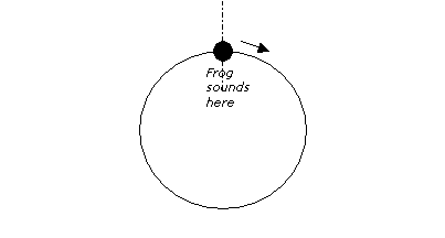
Figure 1 – Cyclical frog chirping

Whenever the ball reaches the apex of the circle, i.e. 12 o’clock, the frog croaks. The speed of the ball travelling around the circle affects the frequency of the frog call. Now, imagine two frogs in this way:

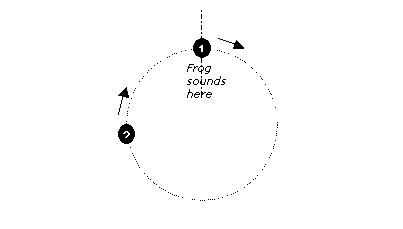
Figure 2 – Two frogs calling

From this diagram we can see that frog 2 will sound a little after frog 1, a delay dependent on their respective speeds (frequency) of cycling (oscillation). If frog 2 is actually faster than frog 1, it will eventually overtake it and take the lead. Extend this example to many more frogs, and the possibility for synchrony or chaos arises:

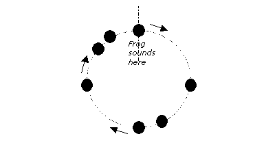
Figure 3 – Many frogs calling

The closer the frog calls are spaced together, the stronger they are synchronised with one another. If the frogs call at the exact same moment – they are completely synchronised. This is the basis for the conceptual model that Synchronous Swamp uses in its generation of sound.

3. The Path to Synchrony - Coupling

How is synchrony achieved in the frog calling model? The answer is coupling, hence the term coupled oscillators. Take the example of the two frogs calling in Figure 1 – in order to sync the two together, the distance between the two must be reduced. Consider that each frog is listening to the other, and that each time it hears its partner call, it speeds up or slows down to compensate, such that the next time it croaks the time delay between the two calls is reduced. In the prior example, frog 1 would slow down and call later than it previously had, while frog 2 would attempt to call earlier, and shorten its period of calling. These two imaginary frogs can then be said to be coupled. Exactly how much and how quickly each frog changes its period of calling to compensate for the distance between them is referred to as the coupling strength. The coupling strength is an important parameter of the Synchronised Swamp installation as it is one of the major factors driving the synchronisation that is seen and heard.

4. The Sync Equation

The playback of sounds in Synchronised Swamp, with a couple of exceptions, is entirely driven by one mathematical relation. At times this equation cannot be heard, or could be mistaken for a random probability distribution, where each sound emitted appears to have been randomly generated over time. The frog sounds are short in duration, so that in large numbers they can form clouds of sound not unlike the experiments of Xenakis [3] who employed Gaussian and Poisson distributions as compositional tools. Xenakis realised that the aggregate of a large number of events can be perceived as an event in its own right. This is where the mass synchronisation generated in Synchronised Swamp comes into play - pockets of synchronised frogs emerge from the soup of particles, as if an invisible attractor were drawing clusters together. Complex rhythms that previously escaped the casual listener begin to emerge. Finally, the avalanche of accumulated synchronisation lashes out in a wave of distributed sound, much like the noise made by the sea rapidly ebbing from a beach carpeted with loose shingles.

The sync equation used is one that was initially formulated by mathematician Yoshiki Kuramoto, based in work done by Art Winfree [4]. It describes a system of n different oscillators. The oscillators have initial starting frequencies that are described by a Gaussian distribution, such that most of the frequencies are clustered together. The equation models a system where every oscillator is coupled to each other. What this means in terms of the frog paradigm, is that every frog is listening to every other frog in the group, and adjusting the timing of its call according to the timing of every other frog, as described above in the section on coupling. In practical terms, this paves the way for a very strong form of sync, given that the frogs in the metaphorical swamp are all seeking to arrive at a common period of calling.

5. The Prototype

The development of Synchronised Swamp began with a prototype of the sync model. It was necessary to establish the correct timing of ‘frog’ calls using the coupled oscillator equation before any aesthetic modifications and experimentation could come into play. Timing, after all, is the cornerstone of this artwork. Should the timing not be accurate, the finer details of the synchronisation process would be lost, or not function at all. The frogs were initially represented as sonic clicks – short clips of sine wave material, and particular attention had to be made towards overlapping sounds which typically occurred as the system slid towards complete synchrony. Detail at the sync point had to be sharp – any sloppy form of synchronisation would dilute the impact and the otherwise strong conceptual grounding. Synchronisation is an important and mysterious phenomenon of nature, and any artistic examination of the process would have to hint at its silent, inexorable background mechanism.

Development began with assigning sound to the “frogs”. The PortAudio library (http://www.portaudio.com), an open source sound API written in C was used to communicate with the computer sound-card hardware. PortAudio is a library that provides streaming audio input and output. It is a cross-platform API that works on Windows, Macintosh, Linux and UNIX running OSS, SGI, and BeOS. PortAudio was chosen for its robustness, obvious portability, availability and ability to manipulate digital sound on a sample-by-sample basis. The portability of PortAudio proved to be invaluable as the application was initially built on an IBM T40 laptop running Linux, then tested on a windows partition using the Windows MME sound driver, and then ported to a desktop PC using the Steinberg ASIO driver, which was necessary to achieve multi-channel output.

The process of playing back sound using PortAudio is initiated through a callback function that is called by PortAudio when audio processing is needed. Once the audio stream is started, the callback function will be called repeatedly by PortAudio in the background. In the callback function audio data is written to the output buffer. Sample playback and DSP manipulation take place in the callback function. While calculations for the sync timing occur elsewhere, the PortAudio callback deals with the overlapping of samples, and implements any additional audio processing before the samples are shunted to the various multiple outputs.

For sound sample loading the open source library Libsndfile (http://www.mega-nerd.com/libsndfile/) was used. Libsndfile is a C library for reading and writing files containing sampled sound of various formats (such as Microsoft Windows .wav format) through one standard library interface. It is released as source code and must be compiled to produce a binary. Libsndfile was chosen for its ability to read and write a large number of file formats and reusability on Linux, UNIX, Windows, MacOS and other platforms.

From the initial sine wave clicks that were used as output, with the introduction of Libsndfile it was straightforward to move forward to using digitally recorded samples. The first sound sample employed was still a very short, high resonance ‘puck’ sound, with an emphasis again on its short duration to enable good perception of the temporal structure of the installation.

Using a Pulsar Scope card and Scope Fusion DSP/routing software, 8 channels of audio output were eventually established. Communicating with the card meant sending interleaved frames of audio to the output buffer, with the number of samples per frame being equal to the number of channels used. In order to evenly distribute the frogs and ensure complete frames of 8 channel audio, the total number of frogs was required to be a multiple of 8. Frogs were therefore cyclically assigned to channels in groups of eight.

6. System Mechanics

It should be noted that the absolute time of the sample-synchronisation process was not calculated, but that instead relative time within the framework of the synchronising system was considered important. In other words, there was no attempt to generate the actual frequencies (e.g. in Hz) of the oscillators, only the relative differences between their phases.

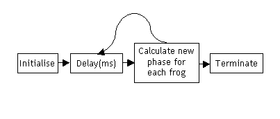
Figure 4 – System Process

From the above diagram it can be seen that the software, after being initialised, remains in an infinite loop until terminated, within which two steps take place. First, the system undergoes a delay (which can be varied over time), and then each frog in the group has its new phase calculated. During the initialisation, each frog is assigned a random phase, as well as an intrinsic frequency, the latter indicating of how often the frog would call if it weren’t under the influence of the sync. This intrinsic frequency is determined using a Gaussian distribution, and the spread of this distribution is also variable.

The formula for calculating the new frog phase is based on the following pseudo code, an implementation of the sync equation as detailed by Strogatz (2000):

theta = coupling_strength * sin((diff/MAX_DEGREES)*2*PI)

new_phase = old_phase + theta;

The variable diff is the phase difference between the current frog and one of the other frogs in the system. In the global approach where there are no constraints, the current frog is compared with all the other frogs in the system, leaving theta to be calculated that many times. The result of the theta equation is to minimise the gap between the current frog and the frog it is being compared with. As a result of this minimisation being employed throughout the entire group of sounding creatures, the system moves towards synchronisation.

7. Unravelling Sync

Experiments with the prototype proved that synchronization did indeed take place. In fact, it proved a little too effective. The global approach where every frog is listening to every other frog, and changing its phase accordingly, resulted in a fast, binding sync. The system synchronized too quickly, even with the most disorganized mob. While the process of sync is a fascinating phenomenon, much of the actual thrill is derived from witnessing a chaotic mess achieve order. Once order has been attained, the system becomes repetitive and less interesting. Oddly enough, after having initially desired to attain sync, it then became imperative to unravel and delay the sync.

Essentially three techniques were used to delay or counter synchronization. Firstly, the most obvious candidate was the coupling strength. The strength of the coupling between elements in the group had a remarkable effect on the speed of synchronization. However, using the initial model, the coupling strength remained too sensitive. Only within a fraction of its range would the system achieve a slow sync. Below this range was chaos, and above, iron clad order. This sensitivity was further reduced by widening the spread of intrinsic frog frequencies. With staggered, widely varying speeds within the group, sync was harder to achieve. Again, though, this suffered the same sensitivity issues as before, albeit abated. Turning back to the literature for inspiration, Kuramoto [5], whose mathematical model this project is based on, had tried to achieve sync using a ring of connectivity with oscillators arranged in a circle. He and his colleagues found that a ring of dissimilar oscillators could not easily achieve widespread synchrony – small groups of neighbours only would tend to cycle together. Implementing this into the Synchronised Swamp was straightforward and quickly accomplished, with a successful outcome. The “frogs” now settled into a shifting sound-scape of lopsided rhythms, with small pockets of repetition. It was as if several groups were simultaneously vying for sync, destabilising the system into a never ending contest for supremacy.

8. Synthetic Sync

Satisfied with the timing, the aesthetics of the swamp were now ready to be developed. After much experimentation, five samples made up the bank of sounds used in the swamp. These were both synthetic and recorded samples of frog and insect-like sounds, edited and drawn from two main sources – sample CDs and the internet. To provide sonic variation, samples were incrementally pitched shifted, beginning from below the root sample to several octaves up (the range being dependent on the total number of frogs). The already fairly short recording now degenerated into rasping and popping twittering – perfect for the swamp.

For additional variation, an oscillating and panning grain based effect developed through experimentation was arbitrarily applied to the first 16 frogs. The result was to produce an uncanny cricket-like sound that hopped in a lively fashion from speaker to speaker. Further trial and error lead to two favoured frog populations, one of 32 frogs and one of 256. The former offered good resolution and clarity, with simple, crisp rhythms, while the larger group demonstrated an animated alternative – a bubbling soup of particles, swirling and giddy under the influence of the power of sync, producing an odd but hypnotic sensation of an organic system moving inexorably forward towards some infinite point, driven by an inexhaustible kinetic dynamic.

References

[1] Bagla, P. (1999) Behaviorists Listen In as Animals Call and Croak, in Science Magazine, Volume 285, 3^rd September 1999, pp 1480-1481.

[2] Narins, Peter M. (1995) Frog Communication, in Scientific American, Volume 273, Issue 2, August 1995, p78.

[3] Roads, C. (2001) Microsound, Cambridge, Massachusetts: MIT Press.

[4] Strogatz, S. (2000) From Kuramoto to Crawford: exploring the onset of synchronization in populations of coupled oscillators, in Physica D, Volume 143, Issue 1-4: Nonlinear Phenomena, pp 1-20.

[5] Strogatz, S. (2003) Sync: The Emerging Science of Spontaneous Order, New York, Hyperion.